Insights into Molecular Dynamics Simulations and Force Fields

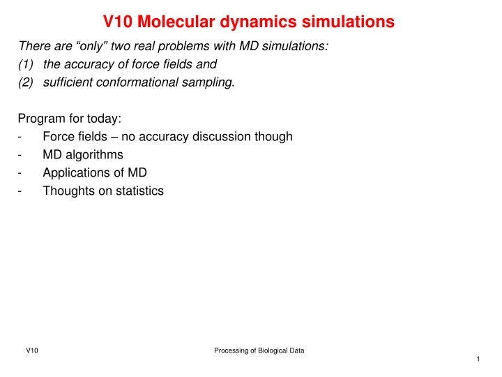
V10 Molecular dynamics simulations There are only two real problems with MD simulations: (1) the accuracy of force fields and (2) sufficient conformational sampling. Program for today: - Force fields no accuracy discussion though - MD algorithms - Applications of MD - Thoughts on statistics V10 Processing of Biological Data 1

Molecular dynamics (MD) simulations MD simulations are nowadays a major technique to study biomolecules in terms of - structure - dynamics, - thermodynamics and - their interaction with other biomolecules. An MD simulation computes the behavior of a molecular system over time. Trajectories of MD simulations contain detailed information on the fluctuations and conformational changes of proteins and nucleic acids. MD simulations are also used by X-ray crystallographers and NMR experimentalists to determine structures, i.e. to generate conformations that match the experimental data. V10 Processing of Biological Data 2

Dynamic processes in biomolecules Local movements (spatial dimensions 0.01 to 5 , time scales 10-15 to 10-1 s) atomic fluctuations movements of side chains movements of loops Movements of rigid bodies (1 to 10 , 10-9 to 1s) movements of alpha-helices Domaim movements (hinge bending) movements of protein subunits Large scale movements (> 5 , 10-7 to 104 s) Helix coil transitions Dissociation/association reactions Folding and unfolding processes V10 Processing of Biological Data 3

Molecular mechanics with empirical force fields There exist specialized force fields for Water (simple molecule, but yields very complicated solution phenomena) and other solvents such as methanol, CHCl3, etc Proteins/peptides Nucleic acids (DNA, RNA) Phospholipids Polymers, sugars Metal atoms, inorganic and bioinorganic substances, (metals are difficult to model with force fields due to d-orbitals -> spatial anisotropy is important for coordination) 3. Vorlesung SS 2006 Computational Chemistry 4

Force field energy = steric energy E steric= covalent (bonded) interactions + non-covalent (nonbonded) interactions XX = E bonds + E angles+ E torsions+ E bonds-angles + ... + X E van-der-Waals+ E electrostatic+ E h-bonds + Eother... = + + + + E E E E E E stretch bend tors vdW ES ( ) ( ) ( ) ( ) ij ijk k k 2 2 ( ) ( ) ij ijk = + r r 0 0 ij ij 2 2 ( ) ( ) bonds ij angles ijk ( 1 ) ( ) ijkl k 2 ( ) ijkl + + ) ( ijkl cos( n 0 2 ( ) torsions ijkl A B q q 1 pairs pairs ( ) ( ) ij ij i r j + + 12 6 4 r r ( ) ( ) ij ij 0 ij ij ij 3. Vorlesung SS 2006 Computational Chemistry 5

Bond stretching modes from vibrational spectroscopy 1= 3657 cm-1 symmetric stretch vibration 2= 3776 cm-1 asymmetric stretch vibration 3= 1595 cm-1 bending vibration Normal modes of a water molecule [Schlick, Fig. 8.1] Asymmetric stretch vibration is energetically more demanding than symmetric stretch vibration ( higher wave number). Bending vibration requires least amount of energy. Bond vibrations are only little coupled to remaining dynamics freezing bond lengths in simulations (SHAKE, LINCS) allows longer time steps 3. Vorlesung SS 2006 Computational Chemistry 6

In-plane and out-of-plane bending 2 types of bending vibrations in the plane 2 types of bending vibrations out of the plane grey atoms: reference position of the molecule. black atoms: position after displacement. In the wagging mode (bottom left), both atoms move toward the observer. In the twisting mode (bottom right) one atom moves toward the observer, the other atom moves away from the observer. 3. Vorlesung SS 2006 Computational Chemistry 7

Torsional energy Etorsion= 0.5 V1(1 + cos ) + 0.5 V2(1 + cos 2 ) + 0.5 V3(1 + cos 3 ) 2,5 2,5 2 2 1,5 1,5 Energy Energy 1 1 0,5 0 0,5 0 30 60 90 120 150 180 210 240 270 300 330 360 Torsion Angle 0 0 30 60 90 120 150 180 210 240 270 300 330 360 Torsion Angle 5 Energy 0 0 30 60 90 120 150 180 210 240 270 300 330 360 Torsion Angle 3. Vorlesung SS 2006 Computational Chemistry 8

Rotational barrier of butane: sum of 2 terms (1+ cos ) + cos3 2,5 2 1,5 Energy 1 0,5 0 0 30 60 90 120 150 180 210 240 270 300 330 360 Torsion Angle 3. Vorlesung SS 2006 Computational Chemistry 9

Non bonded interactions Possibilities for parametrization: Uncharged noble atoms interact only via van der Waals (vdW) forces. [Leach] 3. Vorlesung SS 2006 Computational Chemistry 10

Van der Waals interactions vdW interactions are based on the overlap of the electron clouds of 2 atoms (electronic correlation). One can think of this as an induced dipole-dipole interaction. At close distances, both electrons repel eachother strongly. At medium distances, the interaction is attractive. At large distances, it decays with 1/r6. A B ( ) ( ) ij ij = E It can be modelled as: vdW 12 6 r r ij ij In force fields, Aiiand Biiare fitted against some experimental data for each atom type. 3. Vorlesung SS 2006 Computational Chemistry 11

Van der Waals interaction Analogous representation: 12 6 = 4 EvdW r r with the collision diameter and the depth of the energy minimum . (One can also represent the potential by rm= r*. EvdW A B = 0 Taking ( ) ( ) ij ij = E r By comparison with vdW 12 6 r r ij ij 1 = 2 mr 6 yields = = 12 12 m r 4 A r one obtains: = = 6 6 4 2 B m 3. Vorlesung SS 2006 Computational Chemistry 12

Combination rules To describe arbitrary interactions Eijbetween two different atom types one often uses the combination rule named after Lorentz-Berthelot: or AB= ( AA+ BB) Geometric: r*AB= (r*AA+ r*BB) = AB A B 3. Vorlesung SS 2006 Computational Chemistry 13

Electrostatic interactions: Coulomb law 0 4 pairs r q q 1 i r j = E ES ( ) ij ij 0= 8,854 10-12As/Vm : electrical field constant r: relative dielectric constant of the medium e.g. 2 in the interior of proteins and in membranes 80 in water In molecular mechanics one typically uses r= 1 for the interaction between all atoms that are explicitly modelled Neglecting solvent molecules saves a lot computing time. Then, the solvent effect can be modelled by a distance-dependent dielectric constant r= r. The idea of this is: if solvent molecules were present, they would orient themselves to screen all pairwise interactions. qiand qjare suitable atomic point charges 3. Vorlesung SS 2006 Computational Chemistry 14

Force field parametrization Covalent terms - Bond lengths and -angles - Dihedral (torsional) angles - force constants X-ray structures of small molecules (CSD) stereo chemistry e.g. from infrared vibrational spectroscopy This approach has only difficulties if cross terms are used in the force field. Most accurate force field: Merck force field MMFF, that was parametrized against accurate quantum chemical calculations. Non covalent terms Are tuned so that conformations are correctly sampled and energy differences of E und G are correctly computed. 3. Vorlesung SS 2006 Computational Chemistry 15

Take home message 1: force fields are horror Molecular mechanics method is a serious simplification. This is only historically justified because computing resources were severly limited in the old days . - Developers of different empirical force fields split up energy terms in very different ways: - Some implement any possible sort of interaction, - others use only 5-10 terms. Missing terms need to be compensated by ad hoc parametrisions. - Values of the potential function have no physical meaning, but depend on potential function and parameters. 3. Vorlesung SS 2006 Computational Chemistry 16

Take home message 2: force fields are practically useful Relative energy difference of isomers is predicted quite well by MM force fields MM force fields are well suited for conformational analyses (though peptides are particularly tricky ) Force fields enable simple calculation intermolecular interactions. Force field calculations are very efficient Only force fields allow treating large systems with 100.000 1.00.000 atoms, and even their dynamics. 3. Vorlesung SS 2006 Computational Chemistry 17

History of MD simlations 1957/1959: First MD simulation of hard spheres mimicking fluids (Alder & Wainwright) 1964 first simulation with realistic potential for liquid argon (Rahman, 1964) 1974 first MD simulation of water (Stillinger and Rahman, 1974) 1977 first MD simulation of the protein BPTI (McCammon, et al, 1977). 1977 SHAKE algorithm (to freeze bond lengths) 1983 CHARMM, AMBER force fields 1984 free energy calculations 1985 Car-Parrinello MD 1987 Gromos87 force fields since 1990 QM/MM methods, e.g. of enzymatic reactions (Noble prize 2013) 1992 Ewald method (efficient FFT computation of long-range electrostatics) 1990ies: MD simulation on parallel processos larger systems Alder, B. J. and Wainwright, T. E. J. Chem. Phys.27, 1208 (1957) Alder, B. J. and Wainwright, T. E. J. Chem. Phys.31, 459 (1959) Rahman, A. Phys. Rev. A136, 405 (1964) Stillinger, F. H. and Rahman, A. J. Chem. Phys.60, 1545 (1974) McCammon, J. A., Gelin, B. R., and Karplus, M. Nature (Lond.)267, 585 (1977) V10 Processing of Biological Data 18

A simple MD package program md call init t = 0 do while (t.lt.tmax) call force(f,en) call integrate(f,en) integrate equations of motion t = t + delta call sample enddo stop end Initialization MD loop compute forces compute averages after [Frenkel, Smit 1996] V10 Processing of Biological Data 19

Initialization in an MD program subroutine init sumv=0 sumv2=0 do i=1,npart x(i)= lattice_pos(i) v(i)=(ranf()-0.5) sumv=sumv+v(i) sumv2=sumv2+v(i)**2 enddo sum=sumv/npart sumv2=sumv2/npart fs=sqrt(3*temp/sumv2) do i=1,npart v(i)=(v(i)-sumv)*fs xm(i)=x(i)-v(i)*dt enddo return end Initialization place particles on lattice (or read starting coordinates) assign random velocities velocity of the center of mass (CMS) kinetic energy velocity of the CMS mean squared velocity scaling factor for particle velocities set desired kinetic energy - set CMS velocity to zero position at previous time step - (is needed for integration algorithm) after [Frenkel, Smit 1996] V10 Processing of Biological Data 20

periodic boundary conditions (PBC) Using PBC enables simulations with fairly small particle numbers, whereby particles are subject to forces like in solution. The coordinates of the periodic copies are obtained by simply translating the coordinates of the particles in the central box. Central particles feel interactions with other central particles or with their periodic copies. 2-dimensional box. A suitable cut-off ensures that a central particle cannot interact both with another central particle and with one of its copies. central box is surrounded by 8 neighbors For a cubic box: cut-off < box/2 nach [Frenkel, Smit 1996] V10 Processing of Biological Data 21

Computation of forces subroutine force(f,en) en=0 do i=1,npart f(i)= 0 enddo do i=1,npart-1 do j=i+1,npart xr=x(i)-x(j) xr=xr-box*nint(xr/box) r2=xr**2 if (r2.lt.rc2) then r2i=1/r2 r6i=r2i**3 ff=48*r2i*r6i*(r6i-0.5) in this example:Lennard-Jones potential f(i)=f(i)+ff*xr f(j)=f(j)-ff*xr en=en+4*r6i*(r6i-1)-ecut endif enddo enddo return end Initialization set forces to 0 Loop over all pairs of particles (atoms) compute distance of particles i and j periodic boundary conditions check whether distance < cut-off Update of forces Update of energy nach [Frenkel, Smit 1996] V10 Processing of Biological Data 22

Taylor expansion Let function f be n+1 times differentiable in an interval [x0- , x0+ ]. Then, the Taylor expansion applies in this interval: ( )( v x 1 n f x ( ) x ) ( ) x = + 0 f x x R 0 n ! = 0 mit ( ( ) )( + + x n 1 n 1 + def f x x x 1 , 0 ( ) x ) = + 1 n 0 0 , R x x ( ) 0 n + 1 1 ! n V10 Processing of Biological Data 23

Integration of the equations of motion Taylor expansion of the particle coordinates r(t) ( ) 2 t F ( ) 3 F t t ( ) ( ) t ( ) t + = + + + + 2 4 r r v r , t t t t O t ! 3 t m ( ) 2 m ( ) 3 ( ) ( ) t ( ) t = + + 2 4 r r v r t t t t O t ! 3 Summation gives Subtractio + r n r yields ( ) m ( ) ( ) F t ( ) ( ) ( ) t ( ) ( ) ( ) t = + 3 + + = + + v 2 4 2 t t t t t O t r r r 2 t t t t t O t and or ( ) 2 ( ) ( ) m + ( ) r r t t t t F t ( ) t ( ) ( ) t ( ) = + 2 v + + O t 2 r r r 2 t t t t t t This is the Verlet algorithm. Velocities do not show up explicitly, but can be computed from the trajectory. V10 Processing of Biological Data 24

Leap-frog algorithm Leap-frog ( Bocksprung- ) algorithm using r ( ) t ( t ) 2 r t t t v t ( ) t ( ) t 2 + r r t t t + v t yields 2 t ( ) ( ) t + = + + r r v t t t t The update of the velocities is: ( ) t ( ) t 2 + r r t t t + = v t ( ) t ( t ) ( ) t ( ) t 2 + r r r r t t t t t = + v t ( ) m algorithm 2 F t t = + v Verlet t t as the yields ( ) m ( ) ( ) t ( ) + + F r r r 2 t t t t t t = t V10 Processing of Biological Data 25

Integrate equations of motion subroutine integrate(f,en) sumv=0 sumv2=0 do i=1,npart xx=2*x(i)-xm(i)+delt**2*f(i) v(i)=(xx-xm(i))/(2*delt) sumv=sumv+v(i) sumv2=sumv2*v(i)**2 xx(i)=xx enddo temp=sumv2/(3*npart) etot=(en+sumv2)/(2*npart) return end integrate equations of motion MD loop Verlet algorithm velocities CMS velocity total kinetic energy position update current temperature total energy per particle nach [Frenkel, Smit 1996] V10 Processing of Biological Data 26

Example 1: Fast-folding proteins fold/unfold in MD simulations - 12 protein domains (10 to 80 amino acids) without disulfide bonds or prosthetic groups. - Different topologies: -helical, sheet and mixed / . - MD simulations used a single force field and included explicitly represented solvent molecules. Fig shows folded structure obtained from simulation (blue) superimposed on the experimentally determined structure (red), Lindorff-Larsen, , David E. Shaw Science (2011) 334, 517-520 V10 Processing of Biological Data 27

Fast-folding proteins fold/unfold in MD simulations For each of the 12 proteins, 1 to 4 simulations were performed, each between 100 s and 1 ms long. For each protein, at least 10 folding and 10 unfolding events were observed. In ~8 ms of simulation, more than 400 folding or unfolding events were observed. For 8 of the 12 proteins, the most representative structure of the folded state fell within 2 root mean square deviation (RMSD) of the experimental structure. Lindorff-Larsen, , David E. Shaw Science (2011) 334, 517-520 V10 Processing of Biological Data 28

Example 2: How do voltage-dependent K+ channels work? Hodgkin and Huxley discovered that voltage-regulated ion flow underlies nerve conduction. Voltage-sensing domains (VSD) control the activity of voltage-gated K+, Na+, and Ca2+channels, shifting these proteins between activated and deactivated states in response to changes in transmembrane voltage. Different mechanistic models have been proposed to describe how conserved arginine and lysine gating-charge residues on a VSD transmembrane helix (S4) couple with the electric field to gate ion channel conduction. Show movies 1 and 7 at http://science.sciencemag.org/content/suppl/2012/04/11/336.6078.229.DC1 Jensen, David E. Shaw, Science (2012) 336, 229 233. V10 Processing of Biological Data 29

Example 3: Stereoselectivity of the Serotonin 5-HT1AReceptor Q: Why do certain molecules act as activators (agonists) whereas others, with nearly identical structures, act as blockers (antagonists) of GPCRs? Approach: study by MD simulations how two diastereomers (epimers) of dihydrofuroaporphine bind to the serotonin 5-HT1Areceptor and exert opposite effects. Yuan et al. (2016) Angew Chemie Int Ed 55, 8661 V10 Processing of Biological Data 30

Example 3: Stereoselectivity of the Serotonin 5-HT1AReceptor (1) The methyl group at the chiral center of the agonist molecule contacts Phe3626.52of the receptor through hydrophobic interactions, thereby resulting in a rotamer switch of the phenyl group of this residue. (2) This first movement induces structural changes in the transmission switch, including the central residue in this switch, the highly conserved Trp3586.48. (3) This opens a gate, followed by opening of the 3 7 lock of the receptor, thereby (4) eventually allowing diffusion of water molecules from the bulk extracellular phase towards the central cytoplasmic internal space of the receptor. (5) The successive movement of water molecules into the receptor induces structural changes in TM5, TM6, and TM7, first bending and then rotation, (6) This finally enables the binding and activation of a G protein at the intracellular site of the receptor. Are the observations of the MD simulations statistically significant? Yuan et al. (2016) Angew Chemie Int Ed 55, 8661 V10 Processing of Biological Data 31

Example 3: Stereoselectivity of the Serotonin 5-HT1AReceptor 3 1.2 s all-atom MD simulations were performed for both the agonist- bound and the antagonist-bound 5- HT1Areceptor. All 3 agonist-simulations showed the conformational transitions (feature ), but none of the antagonist-simulations. According to the hypergeometric test, N = 6, K = 3 n = 3, k = 3 this is statistically significant (p = 0.05). Yuan et al. (2016) Angew Chemie Int Ed 55, 8661 V10 Processing of Biological Data 32

Example 4: Autocorrelation of observables in trajectory All 3 correlation functions drop smoothly to zero within 200 ps a 100 ns simulation contains many independent samples. BUT: more complicated systems/variables have much longer autocorrelation times! The populations for the 3 states are 0.78, 0.10, and 0.13 for trans, g+, and g . State autocorrelations computed from 100 ns butane simulations. The central torsion was labeled as either trans, g+, or g . ? ? ? BUT g+ and g are physically identical. They should have the same population! even a very long simulation of a very simple system is incapable of estimating populations with high precision. ? ? + ? ? ?? ??? = 2 Grosfield (2009) Annu Rev Comput Chem 5, 23 V10 Processing of Biological Data 33