Insights on Utility-Based Risk Ranking Procedures

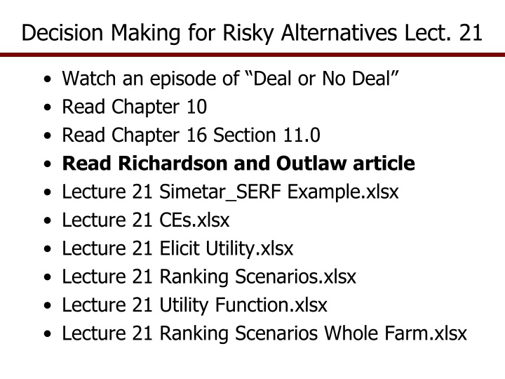
Decision Making for Risky Alternatives Lect. 21 Watch an episode of Deal or No Deal Read Chapter 10 Read Chapter 16 Section 11.0 Read Richardson and Outlaw article Lecture 21 Simetar_SERF Example.xlsx Lecture 21 CEs.xlsx Lecture 21 Elicit Utility.xlsx Lecture 21 Ranking Scenarios.xlsx Lecture 21 Utility Function.xlsx Lecture 21 Ranking Scenarios Whole Farm.xlsx

Utility Based Risk Ranking Procedures Utility and risk are often stated as a lottery Assume you own a lottery ticket that will pay you $10 or $0, with a probability of 50% Risk neutral DM will sell the ticket for $5 Risk averse DM will sell ticket for a certain (non- risky) payment less than $5, say $4 Risk loving DM will sell if paid a certain amount greater than $5, say $7 Amount of the certain payment to sell the ticket is DM s Certainty Equivalent or CE Risk premium (RP) is the difference between the CE and the expected value RP = E(Value) CE RP = 5 4

Utility Based Risk Ranking Procedures CE is used everyday when we make risky decisions We implicitly calculate a CE for each risky alternative Deal or No Deal game show is a good example Player has 4 unopened boxes with amounts of: $5, $50,000, $250,000 and $0 Offered a certain payment (say, $65,000) to exit the game, the certain payment is always less than the expected value (E(x) =$75,001.25 in this example) If a contestant takes the Deal, then the Certain Payment offer exceeded their implicit CE for that particular gamble Their CE is based on their risk aversion level

Utility Based Risk Ranking Procedures Utility Utility Function for Risk Averse Person E($) =$5 Income $0 $10 CE($) Risk Averse DM

Ranking Risky Alternatives Using Utility With a simple assumption, the DM prefers more to less, then we can rank risky alternatives with CE DM will always prefer the risky alternative with the greater CE To calculate a CE, all we have to do is assume a utility function and that the DM is rational and consistent, calculate their risk aversion coefficient, and then calculate the DM s utility for a risky choice

Ranking Risky Alternatives Using Utility Utility based risk ranking tools in Simetar Stochastic dominance with respect to a function (SDRF) Certainty equivalents (CE) Stochastic efficiency with respect to a function (SERF) Risk Premiums (RP) All of these procedures require estimating the DM s risk aversion coefficient (RAC) as it is the parameter for the Utility Function

Suggestions on Setting the RACs Anderson and Dillon (1992) proposed a relative risk aversion (RRAC) definition of 0.0 risk neutral 0.5 hardly risk averse 1.0 normal or somewhat risk averse 2.0 moderately risk averse 3.0 very risk averse 4.0 extremely risk averse (4.01 is a maximum) Rule for setting RRAC and ARAC range is: Utility Function Lower RAC Upper RAC Neg Exponential Utility ARAC Power Utility RRAC 0 4/Wealth 0 4.000001

Assuming a Utility Function for the DM Power utility function Use this function when assuming the DM exhibits relative risk aversion RRAC DM willing to take on more risk as wealth increases Or when ranking risky scenarios with a KOV that is calculated over multiple years, as: Net Present Value (NPV) Present Value of Ending Net Worth (PVENW)

Assuming a Utility Function for the DM Negative Exponential utility function Use this function when assuming DM exhibits constant absolute risk aversion ARAC DM will not take on more risk as wealth increases Or when ranking risky scenarios using KOVs for single year, such as: Annual net cash income or return on investments You get the same rankings if you use correct the RACs

Estimate the DMs RAC Calculate RAC Enter values in the cells that are Yellow Lecture 14 Elicit Utility .xls

1. Stochastic Dominance Stochastic Dominance assumes Decision maker is an expected value maximizer Risky alternative distributions (F and G) are mutually exclusive These are two scenarios we simulated Distributions F and G are based on population probability distributions. In simulation, these are 500 iterations for alternative scenarios of a KOV, e.g. NPV First degree stochastic dominance when CDFs do not cross In this case we can say, All decision makers prefer distribution whose CDF is furthest to the right. However, we are not always lucky enough to have distributions that do not cross.

Stochastic Dominance wrt a Function (SDRF) or Generalized Stoch. Dominance SDRF measures the difference between two risky distributions, F and G, at each value on the Y axis, and weights differences by a utility function using the DM s ARAC. 1.0 ----------------------------------------------------------------------------------------------------------------------------------------- P(x) F(x) is blue CDF G(x) is red CDF 0.0 A B NPV for F and G F(x) dominates G(x) for NPV values from zero to A and G(x) dominates from A to B, F(x) dominates for NPV values > B At each probability, calculate F(x) minus G(x) (the horizontal bars between F and G) and weight the difference by a utility function for the upper and lower RACs Sum the differences and keep score of U(F(x)) <?> U(G(x))

Ranking Scenarios with SDRF in Simetar Interpretation of a sample Stochastic Dominance result For all decision makers with a RAC between -0.01 to 0.1: The preferred scenarios are Options 1 and 2 the efficient set If Options 1 and 2 are not available, then Option 3 is preferred Options 4 and 5 are the least preferred Note that Stochastic Dominance resulted in a split decision The Efficient Set has more than one alternative

2. Rank Risky Scenarios Using CE

3. Stochastic Efficiency (SERF) Stochastic Efficiency with Respect to a Function (SERF) calculates the certainty equivalent for risky alternatives at 25 different RAC levels Compare CE of all risky alternatives at each RAC level Scenario with the highest CE for the DM s RAC is the preferred scenario Summarize the CE results for possible RACs in a chart Identify the efficient set based on the highest CE within a range of RACs Efficient Set This is utility shorthand for saying the risky alternative(s) that is (are) the most preferred

Ranking Scenarios with Stochastic Efficiency (SERF) SERF requires an assumption about the decision makers utility function and like SDRF uses a range of RAC s SERF ranks risky strategies based on expected utility which is expressed as CE at the DM s RAC level Simetar includes SERF and calculates a table of CE s over a range of RAC values from the LRAC to the URAC and develops a chart for ranking alternatives

Ranking Scenarios with SERF SERF results point out the reason that SDRF produces inconsistent rankings SDRF only uses the minimum and maximum RACs The efficient set (ranking) can differ from minimum the RAC to the maximum RAC Changing the RACs and re-running SDRF can be slow SERF can show the actual RAC where the decision maker is indifferent between scenarios (this is the BRAC or breakeven risk aversion coefficient) The SERF Table is best understood as a chart developed by Simetar

Ranking Scenarios with SERF Two examples are presented next The first is for ranking an annual decision using annual net cash income Uses negative exponential utility function Lower ARAC = zero Upper ARAC = 4.0/Wealth The second example is for ranking a multiple year decision using NPV variable Uses Power Utility function Lower RRAC = zero Upper RRAC = 4.001

Ranking Risky Annual NCIs with SERF CDF of Annual Net Incomes for Five Risky Alternatives 1 0.9 0.8 0.7 0.6 Prob 0.5 0.4 0.3 0.2 0.1 0 -150000 -100000 -50000 0 50000 100000 150000 200000 Alt 1 Alt 2 Alt 3 Alt 4 Alt 5

Ranking Risky Annual NCIs with SERF

Power Utility Function in SERF

Ranking Risky Alternatives with SERF Interpret the SERF chart as follows The risky alternative that has the highest CE at a particular RAC is the preferred strategy Within a range of RACs the risky alternative which has the highest CE line is preferred If the CE lines cross at that point the DM is indifferent between the two risky alternatives and find a BRAC If the CE line goes negative, the DM would rather earn nothing than to invest in that alternative Interpret the rankings within risk aversion intervals RAC = 0 is for risk neutral DM s RAC = 1 or 1/W is for normal slightly risk aversion DM s RAC = 2 or 2/W is for moderately risk averse DM s RAC = 4 or 4/W is for extremely risk averse DM s

4. Ranking Using Risk Premiums Risk Premium (RP) - calculate the risk premium between each of the scenarios and a base scenario. Risk Premium equals difference between the CE s for the risky scenarios: RPG to F = CEG CEF Rank the risky scenarios based on the RPs Advantage is that the full distribution (F(x) and G(x)) of values for the KOV are compared to each other, based on the decision maker s RAC, i.e., their utility function A wide range of RACs can be tested to allow for a wider range of decision makers given an assumed utility function Base scenario should be the current situation or the scenario picked best by stochastic efficiency (SERF)

Ranking Using Risk Premiums Table The RP Table is calculated like the SERF Table using the same range of 25 RACs The user specifies the base scenario; Option 1 was selected for this example Select the scenario that has highest risk premium for the RAC which best defines the decision maker

Ranking Using Risk Premiums Neg. Exponential Utility Weighted Risk Premiums Relative to Alt 1 Risk Premium decision maker must be paid to accept an inferior scenario 10,000 Alt 4 Based on the Risk Premium, decision maker would pay to move from Base to Alt 4 Alt 3 5,000 - Alt 1 0.000000 0.000050 0.000100 0.000150 0.000200 0.000250 0.000300 0.000350 (5,000) Alt 5 (10,000) (15,000) Alt 2 (20,000) ARAC Alt 1 Alt 2 Alt 3 Alt 4 Alt 5 Risk premiums are presented relative to a base scenario, Alt 1, above Alt 4 is preferred for all risk averse decision makers. Distance between Red line and Base line, $18,347, is how much a risk averse decision maker would pay to move from Alt 2 to Alt 1. Risk averse decision makers prefer Alt 4 to Alt 1 and would pay about $8,000 to gain Alt 4 over Alt 1.

Roys Safety First Rule Roy (Econometrica, 1952) Select the strategy which minimizes the chance of falling below a critical level of net cash income Rank risky alternatives based on the scenario with the smallest probability of low net cash incomes This is essentially a two light Stop Light chart

Roys Safety First Rule A Roy s Safety First Rule presented as the probability of NCIi < target each year i With Roy s Rule, can calculate the probability of a low net cash income for two or more consecutive years, as: =IF(AND(NCI1<0, NCI2<0),1,0) =IF(AND(NCI2<0, NCI3<0),1,0) =IF(AND(NCI3<0, NCI4<0),1,0) =IF(AND(NCI4<0, NCI5<0),1,0) Repeat the =IF(AND()) statement for all years 2-T and summarize the counter variables for all iterations Roy s probability is sum for all of the =IF(AND()) values divided by (No. Years 1) * No. Iterations If 10 years and 500 iterations the denominator is 4,500 representing all possible sample observations that could be 1

Roys Safety First Rule Roy's Probability 0.335556 =SUM(M9:U108)/900 =IF(AND(B9<0,C9<0),1,0) Roys 1-2 Roys 2-3 Roys 3-4 Roys 4-5 Roys 5-6 Roys 6-7 Roys 7-8 Roys 8-9 0.000 0.000 0.000 1.000 0.000 0.000 0.000 0.000 0.000 0.000 0.000 0.000 0.000 0.000 0.000 0.000 0.000 0.000 0.000 0.000 0.000 0.000 0.000 0.000 0.000 1.000 1.000 1.000 1.000 1.000 1.000 1.000 0.000 0.000 0.000 0.000 0.000 0.000 0.000 0.000 Iteration Roys 9-10 0.000 0.000 0.000 0.000 0.000 0.000 0.000 1.000 0.000 1.000 1 2 3 4 5 6 7 8 9 1.000 0.000 0.000 0.000 0.000 0.000 1.000 1.000 0.000 0.000 0.000 0.000 0.000 0.000 0.000 0.000 0.000 1.000 0.000 1.000 0.000 0.000 0.000 0.000 0.000 0.000 0.000 1.000 0.000 1.000 0.000 0.000 0.000 0.000 0.000 0.000 0.000 1.000 0.000 1.000 10 The scenario was simulated 100 iterations Net cash income is for 10 years Roy s values are for 2 consecutive years with negative NCI Roy s Probability is the sum of the =IF(AND()) counter variables divided by 900, which is = 9 * no. iterations

Roys Safety First Rule StopLight Chart for Probabilities Less Than 0.000 and Greater Than 1.000 100% 0.14 0.20 90% 0.00 0.30 0.33 0.37 0.39 80% 0.00 0.40 0.44 0.45 70% 0.00 0.00 0.00 0.00 60% 0.00 0.00 0.00 50% 0.86 40% 0.80 0.70 0.67 0.63 0.61 30% 0.60 0.56 0.55 20% 10% 0% Roys 1-2 Roys 2-3 Roys 3-4 Roys 4-5 Roys 5-6 Roys 6-7 Roys 7-8 Roys 8-9 Roys 9-10 The Stop Light displays the probabilities of having two years of negative NCI in a row, years 1 & 2 or Years 3 & 4, etc. Chart developed from the data in the previous overhead, over all 100 iterations The counter variables can be 0 or 1 so not marginal probabilities and thus no yellow in the Stop Light

Additional Ranking Risky Considerations Advanced materials provided as an appendix The following overheads are to good to trash but make the lecture to long They complement Chapter 10 READ CHAPTER 10!!!

Ranking Risky Alternatives X=random income simulated for Alter 1 Y=random income simulated for Alter 2 Level of income realized for either is x or y If risk neutral, prefer Alter 1 if E(X) > E(Y) In terms of utility theory, prefer Alter 1 iff E(U(X)) > E(U(Y)) Given that expected utility is calculated as E(U(X)) = P(X=x) * U(x) for all levels x where P(X=x) is probability income equals x

Ranking Risky Alternatives Each risky alternative has a unique CE once we assume a utility function or U(CE) = E(U(X)) Constant absolute risk aversion (CARA) means that if we add $1 to each outcome we do not change the ranking If a bet pays $10 or $0 with probability of 50% it may have a CE of $4 Then if a bet pays $11 or $0 with Probability of 50% the CE is greater than $4 CARA is a reasonable assumption and it allows us to demonstrate risk ranking

Ranking Risky Alternatives A CARA utility function is the negative exponential function U(x) = A - EXP(-x r) A is a constant to convert income to positives r is the ARAC or absolute risk aversion coefficient x is the realized income for the alternative EXP is the exponent function in Excel We can estimate the decision maker s RAC by asking a series of questions regarding gambles

Ranking Risky Alternatives Calculate Utility for a random return or income given a RAC U(x) = A EXP(- (x+scalar) * r) Let A = 1000 to scale all utility values to positive Can try different RAC values such as 0.001 Lecture 15

Alternative RACs Lecture 15

Add or Subtract a Constant $ Amount Lecture 15

Ranking Risky Alternatives Three steps in Utility Analysis 1st convert the monetary payoffs to utility values using a utility function as U(X) =A-EXP(-x*r) and repeat this step for Y 2nd calculate the expected value of U(x) as E(U(X)) = P(X=x) * [A-EXP(-x*r)] Repeat this step for Y 3rd convert the E(U(X)) and the E(U(Y))to a CE CE(X) > CE(Y) means we prefer X to Y based on the DM ARAC of r and the utility function and the simulated Y and X values A short cut is to calculate CE directly for a decision makers RAC Simetar includes a function for calculating CE =CERTEQ(risky income, RAC)

Ranking Risky Alternatives Lecture 15