Learn how integrated analysis can be applied to stock assessment, combining historical and current data to inform population dynamics and improve understanding of processes for effective management of fish stocks.
Please find below an Image/Link to download the presentation.
The content on the website is provided AS IS for your information and personal use only. It may not be sold, licensed, or shared on other websites without obtaining consent from the author. If you encounter any issues during the download, it is possible that the publisher has removed the file from their server.
You are allowed to download the files provided on this website for personal or commercial use, subject to the condition that they are used lawfully. All files are the property of their respective owners.
The content on the website is provided AS IS for your information and personal use only. It may not be sold, licensed, or shared on other websites without obtaining consent from the author.
E N D
Presentation Transcript
Introduction to Stock Synthesis Richard Methot Senior Scientist for Stock Assessments NOAA Fisheries Seattle, WA Fit to tag recaptures by tag group TG 22 CATCH-AT-OBSERVED "AGE" 5 0 0 0 TG 19 TG 25 Male ending year selectivity for fishery1 Female time-varying selectivity for fishery1 12 5 15 10 4 5 0 0 4 1.0 8 10 3 6 4 0 0 0 2 23+ 4 5 1 2 21 3 5 0 0 0.8 Selectivity, Retention, Mortality 0 0 0 Recruitment 19 1996 2000 2004 1996 2000 2004 1996 2000 2004 3 0 0 0 TG 20 TG 23 TG 26 17 5 10 0.6 15 2 5 0 0 4 2000 15 8 Frequency 1995 3 10 6 2 0 0 0 13 AGE' 2 1990 4 E x p e c te d B ia s -a d ju s t T im e _ s e rie s V irg in & In it 0.4 Year 1985 5 11 1.0 1 5 0 0 1 2 9 0 0 0 0.8 1 0 0 0 1996 2000 2004 1996 2000 2004 1996 2000 2004 1980 Selectivity 7 0.2 0.6 TG 21 TG 24 TG 27 Selectivity Retention Discard mortality 5 0 0 12 1975 0.2 5 0.4 10 80 8 10 60 40 8 3 6 Length (cm) 0 8 20 0.0 6 6 101 4 0 5 0 0 0 1 0 0 0 0 1 5 0 0 0 2 0 0 0 0 2 5 0 0 0 3 0 0 0 0 3 5 0 0 0 4 0 0 0 0 F e m a le S p a w n in g B io m a s s 4 4 2 60 52 46 40 34 SIZE 28 22 16 0 20 40 60 80 2 2 0 0 0 Length bin (cm) 1996 2000 2004 1996 2000 2004 1996 2000 2004 Year
Objectives of stock assessment CATCH COMMERCIAL, RECREATIONAL, BYCATCH (OBSERVERS) ABUNDANCE NOAA VESSEL and CHARTER SURVEYS, FISHERY CATCH RATE BIOLOGY AGE, GROWTH, MATURITY ADVANCED MODELS HABITAT CLIMATE ECOSYSTEM MANMADE STRESS POPULATION MODEL Calculates time series of Fish Abundance and Mortality SOCIOECONOMICS STATUS Overfishing? Overfished? FORECAST Annual Catch Limit
Integrated Analysis Long time series of quality catch-at-age and index data are often not available. In response we may: Truncate time series to shorter period; losing contrast Create catch-at-age from inadequate data sources; losing sense of imprecision Switch to biomass dynamics model with simple parameters linked to population r & K Integrated analysis can: Span data-poor historical periods and current data-rich era Compare its expected values to a wide variety of data types Link to population dynamics through spawner-recruitment
Bring model to the data Don t transform data to meet rigid model structure Do add processes to model to develop expected values for diverse, lightly processed data Improves understanding of processes Allows simultaneous use of more types of data Statistical properties of data are preserved and transferred to variance of final model results
IA SCAA Comparison SCAA is built around the use of fishery catch-at-age IA is broader and more flexible concept Biological characteristics of catch can be represented by size composition, weight composition, or data-free (biomass dynamics model) Multiple fleets routinely included Predators can be additional sources of mortality Alternative information sources (tag-recapture) Spatial dynamics and movement Less empirical input (such as body wt-at-age) More modeling of processes (growth, size-selectivity, ageing imprecision)
History of Integrated Analysis Fournier & Archibald (1982) provided explicit consideration of errors and use of auxiliary information. CAGEAN (Deriso et al 1985) - 10s of parameters Stock Synthesis (Methot, 1989) -10s to 100s of parameters; FORTRAN & numerical derivatives AD Model Builder (late 1980s) - Computer software to build your own IA, 10s to 1000s of parameters. www.admb-project.org MULTIFAN-CL (1998) - 1000s of parameters (age and size, tag recapture, movement) ASAP (Legault& Restrepo, 1998). A flexible forward age-structured assessment program. Coleraine (Hilborn, Maunder et al, 2000) comparable to ASAP CASAL (Bull et. al 2004; New Zealand) C++ algorithmic stock assessment laboratory); age and size structured, tag recapture, movement GADGET (Begley & Howell, 2004) Globally applicable Area-Disaggregated General Ecosystem Toolbox Stock Synthesis (Methot, 2005; Methot and Wetzel 2013) ADMB-based; size & age based model with spatial structure, gender and growth-morphs
SS History - 1984 Coded in FORTRAN Specific model for anchovy off California Low F, diverse data Temperature effects on maturation and selectivity M = f(predator abundance)
SS History - 1988 Two generalized models coded in FORTRAN 1. SYNL: Size-age structured, allows size and age selectivity, estimates growth parameters 2. SYNA: Age-area structured, empirical body weight input, age selectivity, allows multiple areas with estimable movement rates Target species: west coast groundfish Long-lived, some 50+ yr old fish still in data Weak historical data, except catch, but discarding significant More size than age data; ageing imprecise
SS History 2003 to present Generalized model coded in C++ with ADMB codename: Isabel Merged and expanded features for age/size/area Target species: diverse SS3.24AB (final version), just call it SS SS3.30 now! SS_nextgen in formative stage
Benefits of Stock Synthesis Flexible range of options for many population processes Integrates many sources of data Propagates uncertainty well Works well from very simple to very complex models Widely used Evolving based on decades of development and exploration 11
Benefits of widespread use (of any modeling platform) Bugs less likely to escape notice More comparison with other models More development of associated tools (e.g. for making plots) Facilitates sharing knowledge common language among many scientists more advice on building models easier to understand each others results 12
Stock Synthesis usage hake, about 20 groundfish species cod, flatfish groundfish, surfclam tuna more shrimp groundfish grouper, menhaden anglerfish, sardine, hake tuna, marlin tuna, sharks, small pelagics mackerel, tuna tuna, sharks tuna Many stocks in Chile & Argentina snapper sharks, toothfish, various strange Australian fish 13
Sub-Models of SS Population Model Recruitment, mortality, growth Age and/or size structured Observation Model Derive expected values for data Likelihood-based Statistical Model Quantify goodness-of-fit Algorithm to search for parameter set that maximizes the likelihood Auto-Differentiation Model Builder (ADMB) Cast results in terms of management quantities Propagate uncertainty onto confidence interval for management quantities Parametric bootstrap 14
SS Estimation Procedures Maximize negative logL using ADMB logL is user-weighted composite of components from sources (fleets and surveys) and kinds of data (CPUE, age comp, size comp, etc.) Parameters have user-controlled: min, max, initial value, phase, and optional prior Capable of MLE, MCMC, parametric bootstrap (but no ADMB-RE and no ADMB likelihood profiles) Benchmark (MSY, SPR) and forecast done in sd_phase and mceval_phase
Fundamental Processes 1990 1991 Production: R 1992 1993 1994 Year 1995 1996 1997 1998 1999 2000 0 1 2 3 4 5 6 7 8 9 10 Age Catchability/Selectivity 16
Population Scenario Pop. N-at-Age Sample N-at-Age 35.0 1200 30.0 1000 25.0 800 20.0 15.0 600 10.0 400 Year 5.0 200 0.0 1 3 0 5 7 9 111315171921 1 3 5 7 9 111315171921 Age Age Comp in Final Year 1 0 5 10 15 20 25 What process parameter is causing this deviation? 0.1 OBS Log(fraction) EST 0.01 0.001 17 0.0001
Equally Likely Solutions Change M from .2 to .24 change recruit trend from -.03 to 0.0 1 1 0 5 10 15 20 25 0 5 10 15 20 25 0.1 0.1 OBS OBS Log(fraction) Log(fraction) EST EST 0.01 0.01 0.001 0.001 0.0001 Change dome-selex from -.1 to -.2 0.0001 So, productivity, mortality and selectivity are confounded Attempt to estimate all 3 parameters with one datum would produce parameter correlation near 1.0 Unique solutions require more data with sufficient contrast along relevant dimensions 1 0 5 10 15 20 25 0.1 OBS Log(fraction) EST 0.01 0.001 18 0.0001
SS: No Magic Bullet Allows many kinds of data, but data does not assure contrast Allows many processes to be investigated, but cannot magically remove confounding Fixing parameter values for some processes (M, asymptotic selectivity) will tighten confidence intervals by excluding some alternative explanations for the data that s bad and can be misleading Model with more estimated parameters will have more variance than result from a simpler model that s good, but may be hard to control and understand A fishery interacting with its ecosystem is complex process; our models should not overly simplify this process just because the data are lacking 19
Tuning a Model Result will be a complex weighted average of fit to all included data; Type, contrast and precision of data determine its influence Examine residuals and root mean squared error of fit to data Parsimoniously, add enough process to remove pattern to residuals Judicious re-weighting of inputs to make error assumptions consistent 20
Stock Synthesis Structure NUMBERS-AT-AGE Morphs: gender, settlement time, growth pattern; platoons can be nested within morphs to achieve size- survivorship; AREA Recruits are distributed among areas Age-specific movement between areas FLEET / SURVEY Length-, age-, gender selectivity CATCH F to match observed catch; Catch partitioned into retained and discarded, with discard mortality RECRUITMENT Expected recruitment is a function of total female spawning biomass; Optional environmental input; apportioned among cohorts and morphs; Forecast recruitments are estimated, so get variance PARAMETERS Can have prior/penalty; Time-vary as time blocks, random annual deviations, or a function of input environmental data 21
Types of data Catches Guesstimate on depletion Discards Effort Indices of abundance (fishery and/or survey) Absolute abundance Catch-at-age with ageing error Catch-at-length Age-conditional-on-length Average length-at-age, average weight-at-length Average weight, average length Tagging
Expected Values for Observations 1.0 POPULATION CATCH AT TRUE AGE CATCH AT OBSERVED AGE 0.8 FREQUENCY SELECTIVITY 0.6 0.4 0.2 0.0 25 30 35 40 45 0 5 10 15 20 25 SIZE AGE POPULATION CATCH 60 50 FREQUENCY SIZE-AT-AGE 40 30 POP - SIZE@TRUE AGE CATCH-SIZE@TRUE AGE CATCH-SIZE@OBS. AGE 20 10 0 5 10 15 20 25 10 20 30 40 50 60 70 AGE SIZE 25
Estimation, Benchmarks, Forecasts Sometimes we use a sequence of separate analyses: 1. Estimate population abundance time series 2. Calculate benchmark quantities: target and limit F rates, sometimes based on first fitting spawner-recruitment curve. 3. Forecast future abundance and catch using the target F Integrated Analysis can: Bring all steps into one analytical package Parameter variance from population estimation gets propagated to quantities in forecast Example output: probability that stock abundance will dip below the overfished threshold 5 years into the future, and the standard error of this probability
Fitting to data The goal is estimate the underlying process, given that observations have uncertainty and process has fluctuations Minimize the difference { Prediction
Components of population dynamic models State variables: In the future depend on Current state Parameters Forcing (external shocks) Rules of change (equations) Rules of change Forces (e.g. catches, env.) += 1 S ( , , ) t f S P u t t State variables in next time period State variables (e.g., numbers) Parameters (e.g., growth rate)
Sources of error, e.g. uncertainty Observation error (sampling and measurement error) Process error (dynamics of the resource and the fishery) Model error (model s ability to capture dynamics) Structure of the error (error distributions in likelihood) Estimation error (accuracy of the model parameters) Implementation error (management differs from intended)
Observation error From sampling and measurement error Individual observation error for each piece of data
Model error All models are simplifications We may not fully understand the dynamics of the system There may be important differences between the model and reality It is usually not considered in the stock assessment Absorbed into the process and observation error.
Implementation error Implications due to failure to implement the agreed upon management actions Important in decision analysis and projections Often account for this in Management Strategy Evaluation (MSE)
Model the error Models can assume known observation and/or process error Observation error models regression Process error models assume no or known observation error Models with both errors State-space models Integrated analysis models like SS
Methods Estimation of parameters Moments Least squares Maximum Likelihood (MLE) Bayesian (MCMC) Estimation of uncertainty Delta method Bootstrap Asymptotic theoretical variance (MLE) Likelihood profile (MLE) Posterior distribution (Bayesian)
Data, penalties, priors Penalties and Priors are information about parameters in a model Example: maximum age used to create prior on M Data are information about a derived quantity Expected value for this quantity is derived from model parameters and structure Example: Age composition of catch from a fleet In IA, the expected value for maximum observed age could be derived as a function of M, then observed maximum age could be included as model data Concept of Data and Priors blur; it s all information
Relation to Bayesian analysis Bayesian Analysis (BA) requires prior pdf for all parameters and integrates across this pdf and the posterior pdf to create a posterior pdf of results Information (meta-data) typically used to create priors for a Bayesian analysis can be included as likelihood penalties in IA for some, but not necessarily all, parameters Maximum likelihood (MLE) result is like mode of BA MCMC with IA s parameter penalties produces pdf like that of BA The normal pdf based on the uncertainty of the MLE is comparable to the BA pdf from MCMC, at least in many applications.
Deterministic or stochastic process error Should there be random process error? Deterministic model (no process error) N K = + t N N rN 1 C + t 1 t t t Stochastic model (with process error) = N K + w t N N rN 1 C e t + t 1 t t t where wt is a random variable (typically a normal distribution)
VPA vs. SCAA VPA VPA SCAA SCAA Age -> Age -> Age -> Age -> Year | V V Year | Year | V V Year | Calibrated VPA Estimates abundance of the oldest age and current cohorts Calculates abundance back in time Assumes negligible error in the catch at age F-at-age mostly unconstrained SCAA Estimates initial abundance at age, recruitments, fishing mortality, selectivity Calculates abundance forward in time Allows error in the catch at age 40