Introduction to Classification Trees: CART Algorithm Overview
Classification trees, specifically the CART (Classification and Regression Trees) algorithm, are powerful tools for analyzing data and making predictions. By recursively partitioning data based on predictor values, classification trees aim to create nodes that are as different as possible in terms of outcomes. This process continues until nodes are homogeneous or statistically insignificant. Explore examples like survival on the Titanic to understand how classification trees work and interpret statistics like ROC area and misclassification rate. Learn about tree fitting, partition details, and chi-square values in JMP reports. Gain insights into applying classification trees in practical scenarios involving binary outcomes and potential predictors like glucose level and age.

Download Presentation

Please find below an Image/Link to download the presentation.
The content on the website is provided AS IS for your information and personal use only. It may not be sold, licensed, or shared on other websites without obtaining consent from the author.If you encounter any issues during the download, it is possible that the publisher has removed the file from their server.
You are allowed to download the files provided on this website for personal or commercial use, subject to the condition that they are used lawfully. All files are the property of their respective owners.
The content on the website is provided AS IS for your information and personal use only. It may not be sold, licensed, or shared on other websites without obtaining consent from the author.
E N D
Presentation Transcript
Classification trees CART (classification & regression trees) 1
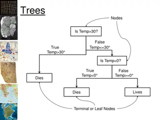
Tree algorithm- binary recursive partitioning The classification tree or regression tree method examines all values of all the predictors (Xs) and finds the best value of the best predictor that splits the data into two groups (nodes) that are as different as possible on the outcome. This process is independently repeated in the two daughter nodes created by the split until either the final ( terminal ) nodes are homogeneous (all observations are the same value, sample size is too small (default: n <5) or the difference between the two nodes is not statistically significant. 2
Survival on the Titanic Outcome (Y): Survival (did not drown) y/n Predictors (Xs): Gender M or F Passenger class 1, 2, 3 Age (years) (Can swim - y/n- don t have this variable) 4
Titanic tree fit stats ROC Area 0.8095 6
Titanic tree fit stats Measure Training Definition Entropy RSquare 0.3042 1-Loglike(model)/Loglike(0) Generalized RSquare 0.4523 (1-(L(0)/L(model))^(2/n))/(1- L(0)^(2/n)) -Log( [j])/n Mean -Log p 0.4628 RMSE 0.3842 (y[j]- [j]) /n Mean Abs Dev 0.2956 |y[j]- [j]|/n Misclassification Rate 0.2116 ( [j] Max)/n n 1309 n Survived Actual No Yes Predicted No 774 242 Yes 35 258 Total 809 500 Acc 95.7% 51.6% 7
JMP tree (partition) details JMP reports chi-square (G2) values for each node. The chi square for testing the significance of a split is computed as G2 test = G2 parent - (G2 left + G2 right). JMP reports the Log Worth rather than the p value (common in genetics) for G2 test Log Worth = - log10(p value) G2 test p value Log Worth 2.71 0.10 1.00 3.84 0.05 1.30 6.63 0.01 2.00 8
Ex: Kidwell -Hemorrhage stroke data, n=89, Y=54 with no hemorrhage, 35 with hemorrhage (binary outcome Y) Potential predictors: Glucose level Platelet count Hematocrit Time to recanalization Coumadin used (y/n) NIH stroke score (0-42) Age Sex Weight SBP DBP Diabetes 9
Hemorrhage model Classification Matrix Actual Category no yes total Predicted Category no yes 11 24 35 56 33 45 9 total 54 89 Sensitivity= 24/35 =69% Specificity= 45/54 =83% Accuracy=76% C = R2 (Hosmer) = 0.606 df=89-5= 84 Deviance/df=72.3/84= 0.861 11
JMP partition details (cont) Can automate making the tree with k fold cross validation option (k=5 by default). Choose this option, then select go . May need to prune tree (remove non significant terminal nodes). 12
Tree Advantages & Disadvantages Advantages: Does not require continuous X to have a linear relation to the logit (does not assume logit= a + bX) May automatically find interactions (X1*X2) so does not require X1 and X2 to be additive ( 1X1 + 2X2) Finds thresholds/cutpoints in X when there is one. Disadvantages: Too complicated/hard to explain if tree too big. Tends to overfit more than logistic (need validation). Not as good as logistic when the relationship with logit really is linear and additive (no thresholds). 13


 details")


")