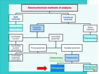
Introduction to Electrochemical Cells and Butler-Volmer Equation

Electrochemical cells play a crucial role in understanding electrode kinetics and models of electrode-electrolyte interfaces. Explore the effects of capacitance current in voltammetry and the Butler-Volmer equation, providing insights into electrode reactions. Learn about charging currents, equilibrium potentials, active surface areas, and more key concepts in electrochemistry.

Download Presentation

Please find below an Image/Link to download the presentation.
The content on the website is provided AS IS for your information and personal use only. It may not be sold, licensed, or shared on other websites without obtaining consent from the author.If you encounter any issues during the download, it is possible that the publisher has removed the file from their server.
You are allowed to download the files provided on this website for personal or commercial use, subject to the condition that they are used lawfully. All files are the property of their respective owners.
The content on the website is provided AS IS for your information and personal use only. It may not be sold, licensed, or shared on other websites without obtaining consent from the author.
E N D
Presentation Transcript
R E C A P R E C A P
1. Electrochemical Cells 2. Models of Electrode/Electrolyte Interface 3. General concepts of Electrode kinetics
Effect of the Capacitance Current in Voltammetry. The reduction of Ferric Chloride is carried out in the presence of 1 M NaCl to eliminate the migration current. (a) 10-5 M Fe3+ Fe3+ + e Fe2+ ild Slope due to ic Current Applied Potential -Ve (b) 10-3 M Fe3+ Fe3+ + e Fe2+ Note that the iE curve in Fig. (a) is recorded at a much higher sensitivity than in Fig. (b). ild Current Applied Potential -Ve
Charging Current or Capacitance Current Note that due to the presence of the electrical double layer a charging or capacitance current is always present in voltammetric measurements.
Butler-Volmer Equation where: I = electrode current, Amps Io= exchange current density, Amp/m2 E = electrode potential, V Eeq= equilibrium potential, V A = electrode active surface area, m2 T = absolute temperature, K n = number of electrons involved in the electrode reaction F = Faraday constant R = universal gas constant = so-called symmetry factor or charge transfer coefficient dimensionless The equation is named after chemists John Alfred Valentine Butler and Max Volmer
Butler Volmer Equation While the Butler-Volmer equation is valid over the full potential range, simpler approximate solutions can be obtained over more restricted ranges of potential. As overpotentials, either positive or negative, become larger than about 0.05 V, the second or the first term of equation becomes negligible, respectively. Hence, simple exponential relationships between current (i.e., rate) and overpotential are obtained, or the overpotential can be considered as logarithmically dependent on the current density. This theoretical result is in agreement with the experimental findings of the German physical chemist Julius Tafel (1905), and the usual plots of overpotential versus log current density are known as Tafel lines. The slope of a Tafel plot reveals the value of the transfer coefficient; for the given direction of the electrode reaction.
Butler-Volmer Equation ( ) 1 nF = exp a i i ia and icare the exhange current densities for the anodic and cathodic reactions ` 0 a RT high at anodic overpotent nF c ial = exp i i ` 0 c RT high at cathodic overpotent ial These equations can be rearranged to give the Tafel equation which was obtained experimentally
Butler Volmer Equation - Tafel Equation RT RT = ln ln i i 0 c c 0 nF 059 nF 059 . 0 c c . = 0 log log at 25 for the C cathodic process i i 0 c c . 0 . 0 n n c c 059 059 = 0 log log at 25 for the C anodic process i i 0 a a equation The + = well n n a a the is known Tafel equation and log a b i 0 . 059 = ln a i o 059 . 0 n = b n
Tafel Equation The Tafel slope is an intensive parameter and does not depend on the electrode surface area. i0 is and extensive parameter and is influenced by the electrode surface area and the kinetics or speed of the reaction. Notice that the Tafel slope is restricted to the number of electrons, n, involved in the charge transfer controlled reaction and the so called symmetry factor, . n is often = 1 and although the symmetry factor can vary between 0 and 1 it is normally close to 0.5. This means that the Tafel slope should be close to 120 mV if n = 1 and 60 mV if n = 2.
Tafel Equation We can write: RT ( ) ( ) = = ln or ln i i b i i 0 0 nF where . 2 303 RT = the = Tafel slope b nF 303 = ln . 2 log i i
Current Voltage Curves for Electrode Reactions Without concentration and therefore mass transport effects to complicate the electrolysis it is possible to establish the effects of voltage on the current flowing. In this situation the quantity E - Ee reflects the activation energy required to force current i to flow. Plotted below are three curves for differing values of io with = 0.5.
Tafel Equation The Tafel equation can be also written as: Where the plus sign under the exponent refers to an anodic reaction, and a minus sign to a cathodic reaction, n is the number of electrons involved in the electrode reaction k is the rate constant for the electrode reaction, R is the universal gas constant, F is the Faraday constant. k is Boltzmann's constant, T is the absolute temperature, e is the electron charge, and is the so called "charge transfer coefficient", the value of which must be between 0 and 1.
Tafel Equation The following equation was obtained experimentally = + log a b i Where: = the over-potential i = the current density a and b = Tafel constants
Tafel Equation Applicability Where an electrochemical reaction occurs in two half reactions on separate electrodes, the Tafel equation is applied to each electrode separately. The Tafel equation assumes that the reverse reaction rate is negligible compared to the forward reaction rate. The Tafel equation is applicable to the region where the values of polarization are high. At low values of polarization, the dependence of current on polarization is usually linear (not logarithmic): This linear region is called "polarization resistance" due to its formal similarity to Ohm s law
Stern Geary Equation Applicable in the linear region of the Butler Volmer Equation at low over- potentials B = i corr R p Where B the = Tafel constant = a c ( ) + 3 . 2 = a c measured the polarisati resistance on R p = E i
Tafel Equation Overview of the terms The exchange current is the current at equilibrium, i.e. the rate at which oxidized and reduced species transfer electrons with the electrode. In other words, the exchange current density is the rate of reaction at the reversible potential (when the overpotential is zero by definition). At the reversible potential, the reaction is in equilibrium meaning that the forward and reverse reactions progress at the same rates. This rate is the exchange current density.
Tafel Equation The Tafel slope is measured experimentally; however, it can be shown theoretically when the dominant reaction mechanism involves the transfer of a single electron that . 2 303 RT = b F T is the absolute temperature, R is the gas constant is the so called "charge transfer coefficient", the value of which must be between 0 and 1.
Levich Levich Equation Equation The Levich Equation models the diffusion and solution flow conditions around a rotating disc electrode (RDE). It is named after Veniamin Grigorievich Levich who first developed an RDE as a tool for electrochemical research. It can be used to predict the current observed at an RDE, in particular, the Levich equation gives the height of the sigmoidal wave observed in rotating disk voltammetry. The sigmoidal wave height is often called the Levich current. In work at a RDE the electrode is usually rotated quite fast (1000 rpm) in order to establish a well defined diffusion layer. The scan rate is relatively slow typically 2-5 mV s-1
Current Voltage Curve at a RDE It is important to remember that in order to determine the diffusion current and the mass transfer coefficient using volatmmetry, excess inert supporting electrolyte must be present to eliminate the migration current
Levich Levich Equation Equation The Levich Equation is written as: where iL is the Levich current n is the number of electrons transferred in the half reaction F is the Faraday constant A is the electrode area D is the diffusion coefficient (see Fick's law of diffusion) w is the angular rotation rate of the electrode v is the kinematic viscosity C is the analyte concentration While the Levich equation suffices for many purposes, improved forms based on derivations utilising more terms in the velocity expression are available.
Levich Equation It is important to note that the layer of solution immediately adjacent to the surface of the electrode behaves as if it were stuck to the electrode. While the bulk of the solution is being stirred vigorously by the rotating electrode, this thin layer of solution manages to cling to the surface of the electrode and appears (from the perspective of the rotating electrode) to be motionless. This layer is called the stagnant layer in order to distinguish it from the remaining bulk of the solution. The act of rotation drags material to the electrode surface where it can react. Providing the rotation speed is kept within the limits that laminar flow is maintained then the mass transport equation is given by the Levich equation.
Levich Equation RDE The Levich equation takes into account both the rate of diffusion across the stagnant layer and the complex solution flow pattern. In particular, the Levich equation gives the height of the sigmoidal wave observed in rotated disk voltammetry. The sigmoid wave height is often called the Levich current, iL, and it is directly proportional to the analyte concentration, C. The Levich equation is written as: iL = (0.620) n F A D2/3 w1/2 v 1/6 C where w is the angular rotation rate of the electrode (radians/sec) and v is the kinematic viscosity of the solution (cm2/sec). The kinematic viscosity is the ratio of the solution's viscosity to its density.
Levich Equation - RDE The linear relationship between Levich current and the square root of the rotation rate is obvious from the Levich plot. A linear least squares fit of the data produces an equation for the best straight line passing through the data. The specific experiment shown, the electrode area, A, was 0.1963 cm2, the analyte concentration, C, was 2.55x10 6 mol/cm3, and the solution had a kinematic viscosity, v, equal to 0.00916 cm2/sec. After careful substitution and unit analysis, you can solve for the diffusion coefficient, D, and obtain a value equal to 4.75x10 6 cm2/s. This result is a little low, probably due to the poor shape of the sigmoidal signal observed in this particular experiment. The kinematic viscosity is the ratio of the absolute viscosity of a solution to its density. Absolute viscosity is measured in poises (1 poise = gram cm 1 sec 1). Kinematic viscosity is measured in stokes (1 stoke = cm2 sec 1). Extensive tables of solution viscosity and more information about viscosity units can be found in the CRC Handbook of Chemistry and Physics.
Cyclic Voltammetry Cyclic Voltammetry is carried out at a stationary electrode. This normally involves the use of an inert disc electrode made from platinum, gold or glassy carbon. Nickel has also been used. The potential is continuously changed as a linear function of time. The rate of change of potential with time is referred to as the scan rate (v). Compared to a RDE the scan rates in cyclic voltammetry are usually much higher, typically 50 mV s-1
Cyclic Voltammetry Cyclic voltammetry, in which the direction of the potential is reversed at the end of the first scan. Thus, the waveform is usually of the form of an isosceles triangle. The advantage using a stationary electrode is that the product of the electron transfer reaction that occurred in the forward scan can be probed again in the reverse scan. CV is a powerful tool for the determination of formal redox potentials, detection of chemical reactions that precede or follow the electrochemical reaction and evaluation of electron transfer kinetics.
Cyclic Voltammetry For a reversible process Epc Epa = 0.059V/n
The The Randles Randles- -Sevcik Sevcik equation Reversible systems equation Reversible systems ( ) 4463 . 0 RT nFvD nFAC ip= ( AC D v n ip 10 687 . 2 = 1 2 ) 5 3 2 1 2 1 2 n = the number of electrons in the redox reaction v = the scan rate in V s-1 F = the Faraday s constant 96,485 coulombs mole-1 A = the electrode area cm2 R = the gas constant 8.314 J mole-1 K-1 T = the temperature K D = the analyte diffusion coefficient cm2 s-1
The Randles-Sevcik equation Reversible systems As expected a plot of peak height vs the square root of the scan rate produces a linear plot, in which the diffusion coefficient can be obtained from the slope of the plot.
Cyclic Voltammetry Stationary Electrode Peak positions are related to formal potential of redox process E0 = (Epa + Epc ) /2 Separation of peaks for a reversible couple is 0.059/n volts A one electron fast electron transfer reaction thus gives 59mV separation Peak potentials are then independent of scan rate Half-peak potential Ep/2 = E1/2 0.028/n Sign is + for a reduction
Cyclic Voltammetry Cyclic Voltammetry Stationary Electrode The shape of the voltammogram depends on the transfer coefficient When deviates from 0.5 the voltammograms become asymmetric -cathodic peak sharper as expected from Butler Volmer eqn. Stationary Electrode
Web Sites Web Sites http://calctool.org/CALC/chem/electrochem/levich http://www.calctool.org/CALC/chem/electrochem/cv1
Tafel Equation The Tafel slope is an intensive parameter and does not depend on the electrode surface area. i0 is and extensive parameter and is influenced by the electrode surface area and the kinetics or speed of the reaction. Notice that the Tafel slope is restricted to the number of electrons, n, involved in the charge transfer controlled reaction and the so called symmetry factor, . n is often = 1 and although the symmetry factor can vary between 0 and 1 it is normally close to 0.5. This means that the Tafel slope should be close to 120 mV if n = 1 and 60 mV if n = 2.
Tafel Equation We can write: RT ( ) ( ) = = ln or ln i i b i i 0 0 nF where . 2 303 RT = the = Tafel slope b nF 303 = ln . 2 log i i


")