Introduction to Hidden Markov Models and Dynamic Programming Techniques

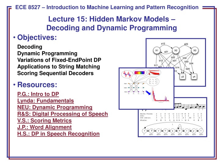
ECE 8443 Pattern Recognition ECE 8527 Introduction to Machine Learning and Pattern Recognition Lecture 15: Hidden Markov Models Decoding and Dynamic Programming Objectives: Decoding Dynamic Programming Variations of Fixed-EndPoint DP Applications to String Matching Scoring Sequential Decoders Resources: P.G.: Intro to DP Lynda: Fundamentals NEU: Dynamic Programming R&S: Digital Processing of Speech V.S.: Scoring Metrics J.P.: Word Alignment H.S.: DP in Speech Recognition

Discrete Hidden Markov Models Elements of the model, ?, are: ?states: ??= ?1,?2, ,?? ?output symbols: ??= ?1,?2, ,?? ? ? ? matrix of transition probabilities: ?11 ?1? ??1 ??? ? ? ? output probabilities: ?11 ?1? ??1 ??? ? = ???= ? ??? + 1 ??? ???? ???= ? ?? ? = ? initial state probabilities (the probability of being in ?? at time 0: ??= ?1,?2, ,?? 0 ??= ? ?? 1,?? 2, ,?? ?. We will refer to the observation sequence as: ??= ?? Note that the transition probabilities only depend on the previous state and the current state (hence , this is a first-order Markov process). ECE 8527: Lecture 15, Slide 1

More Definitions and Comments The state and output probability distributions must sum to 1: ?=1 ???= 1 ? ? ?=1 ???= 1 A Markov model is called ergodic if every one of the states has a nonzero probability of occurring given some starting state. A Markov model is called a hidden Markov model (HMM) if the output symbols cannot be observed directly (e.g., correspond to a state) and can only be observed through a second stochastic process. HMMs are often referred to as a doubly stochastic system or model because state transitions and outputs are modeled as stochastic processes. There are three fundamental problems associated with HMMs: Evaluation: How do we efficiently compute the probability that particular sequences of states was observed? Decoding: What is the most likely sequences of hidden states that produced an observed sequence? Learning: How do we estimate the parameters of the model? ECE 8527: Lecture 15, Slide 2

The Forward Algorithm Fortunately, we can employ a technique similar to what is used in many DSP applications (e.g., the Fast Fourier Transform) to complete this computation using many fewer multiply/adds by storing intermediate results. The probability of being in a state at time ? is given by: 0, 1, ? = 0,? ??????? ?????, ? = 0,? = ??????? ?????, ??? = ??? ??????, ?? ??????. ? where???? ?denotes that the symbol ???was emitted at time ?. This is known as the Forward Algorithm, summarized below in pseudocode: initialize: ? 1 ,? = 0,???, ???, visible sequence ??,? 0 = 1 for: ? ? + 1 ??? = ?=1 ??? 1 ?????? until: ? = ? return: ? ?? ??? end ? ECE 8527: Lecture 15, Slide 3

Decoding (Finding The Most Probable State Sequence) Why might the most probable sequence of hidden states that produced an observed sequence be useful to us? How do we find the most probable sequence of hidden states? Since any symbol is possible at any state, the obvious approach would be to compute the probability of each possible path and choose the most probable: ?? =??? ????? ???? where ?represents an index that enumerates the ??possible sequences of length ?. ? ?? ?? HMM (Viterbi) Decoding: begin initialize: ??? {},? 0 for ? ? + 1,? ? + 1 for ? ? + 1 ??? ??? ?=1 until ? = ? ? ??? ??????? Append ?? ?? ??? until ? = ? return ??? end However, an alternate solution to this ? ??? 1 ??? dynamic programming dynamic programming problem is provided by dynamic programming, and is known as Viterbi Decoding. Viterbi Decoding Note that computing? ??? using the Viterbi algorithm gives a different result than the Forward algorithm. ECE 8527: Lecture 15, Slide 4

Dynamic Programming Consider the problem of finding the best path through a discrete space. We can visualize this using a grid, though dynamic programming solutions need not be limited to such a grid. (u,v) (ik,jk) Define a partial path from (?,?)to (?,?)as an n-tuple: (?,?), ,(?1,?1),(?2,?2), ,(??,??), ,(?,?) The cost in moving from (?? 1,?? 1)to (??,??)is: ? ??,?? (?? 1,?? 1) = (s,t) ??,?? (?? 1,?? 1) +?? ??,?? ?? The cost of a transition is expressed as the sum of transition penalty (or cost) and a node penalty. ? Define the overall path cost as: ? ?,? = ?=1 ? ??,?? (?? 1,?? 1) . Bellman s Principle of Optimality states that an optimal path has the property that whatever the initial conditions and control variables (choices) over some initial period, the control (or decision variables) chosen over the remaining period must be optimal for the remaining problem, with the state resulting from the early decisions taken to be the initial condition. ECE 8527: Lecture 15, Slide 5

The DP Algorithm (Viterbi Decoding) This theorem has a remarkable consequence: we need not exhaustively search for the best path. Instead, we can build the best path by considering a sequence of partial paths, and retaining the best local path. ? ?,? ???,? Only the cost and a backpointer containing the index of the best predecessor node need to be retained at each node. The computational savings over an exhaustive search are enormous (e.g., ?(??) vs. ?(??)) where ? is the number of rows and ? is the number of columns); the solution is essentially linear with respect to the number columns (time). For this reason, dynamic programming is one of the most widely used algorithms for optimization. It has an important relative, linear programming, which solves problems involving inequality constraints. The algorithm consists of two basic steps: Iteration: for every node in every column, find the predecessor node with the least cost, save this index, and compute the new node cost. Backtracking: starting with the last node with the lowest score, backtrack to the previous best predecessor node using the backpointer. This is how we construct the best overall path. In some problems, we can skip this step because we only need the overall score. ECE 8527: Lecture 15, Slide 6

Example Dynamic programming is best illustrated with a string-matching example. Consider the problem of finding the similarity between two words: Pesto and Pita. An intuitive approach would be to align the strings and count the number of misspelled letters: Reference: P I ** t a Hypothesis: P e s t o If each mismatched letter costs 1 unit, the overall similarity would be 3. Let us define a cost function: Transition penalty: a non-diagonal transition incurs a penalty of 1 unit. Node penalty: Any two dissimilar letters that are matched at a node incur a penalty of 1 unit. Let us use a fixed-endpoint approach, which constrains the solution to begin an the origin and end by matching the last two letters ( a and o ). Note that this simple approach does not allow for some common phenomena in spell-checking, such as transposition of letters. ECE 8527: Lecture 15, Slide 7

Discussion Bellman s Principle of Optimality and the resulting algorithm we described require the cost function to obey certain well-known properties (e.g., the node cost cannot be dependent on future events). Though this might seem like a serious constraint, the algorithm has been successfully applied to many graph search problems, and is still used today because of its efficiency. It is very important to remember that a DP solution is only as good as the cost function that is defined. Different cost functions will produce different results. Engineering the cost function is an important part of the technology development process. When applied to time alignment of time series, dynamic programming (DP) is often referred to as dynamic time warping (DTW) because it produces a piecewise linear, or nonuniform, time scale modification between the two signals. ECE 8527: Lecture 15, Slide 8

Variants of DTW: Slope Constraints and Free Endpoints In some applications (such as time series analysis), it is desirable to limit the maximum slope of the best path (e.g., limit the playback speed of a voice mail to a range of [1/2x,2x]. This can reduce the overall computational complexity with only a modest increase in the per-node processing. This can be achieved by implementing different slope constraints. In other applications, such as word spotting, it is advantageous to allow the endpoints to vary. Fig. 1. Constraining the warping path using the: Sakoe-Chiba band (left); Itakura parallelogram (right) This is a special case of general optimization theory. The best path need not start at the lower left or terminate in the upper right of the DP grid. HMMs provide a much better means of achieving this. ECE 8527: Lecture 15, Slide 9

Application: Scoring of Sequential Decoding Systems String Matching: binary similarity measure, equal weighting of error types Ref: bckg seiz SEIZ SEIZ bckg seiz bckg Hyp: bckg seiz BCKG **** bckg seiz **** (Hits: 4 Sub: 1 Ins: 0 Del: 2 Total Errors: 3) Ref: bckg seiz BCKG **** bckg seiz **** Hyp: bckg seiz SEIZ SEIZ bckg seiz bckg (Hits: 4 Sub: 1 Ins: 2 Del: 0 Total Errors: 3) Phonetic String Alignment: using a more sophisticated distance measure based on phonetic similarity Ref: CUT TALL SPRUCE TREES Hyp: HAUL MOOSE FOR FREE Rph: K AX T T ae ** l S P R Y uw s ** ** ** ** T r iy S Hph: ** ** ** HH ae AX l ** ** M ** uw s F OW R ** F r iy ** (Hits: 9 Sub: 3 Ins: 2 Del: 6 Total Errors: 11) Ref: CUT TALL SPRUCE *** TREES Hyp: *** HAUL MOOSE FOR FREE (Hits: 0 Sub: 3 Ins: 1 Del: 1 Total Errors: 5) ECE 8527: Lecture 15, Slide 10

Application: Scoring of Sequential Decoding Systems ECE 8527: Lecture 15, Slide 11

Summary What we discussed in this lecture: Reviewed discrete Hidden Markov Models. Formally introduced dynamic programming. Described its use to find the best state sequence in a hidden Markov model. Demonstrated its application to a range of problems including string matching. Remaining issues: Derive the reestimation equations using the EM Theorem so we can guarantee convergence. Generalize the output distribution to a continuous distribution using a Gaussian mixture model. ECE 8527: Lecture 15, Slide 12