Introduction to Machine Learning: Strategies, Applications, and Types

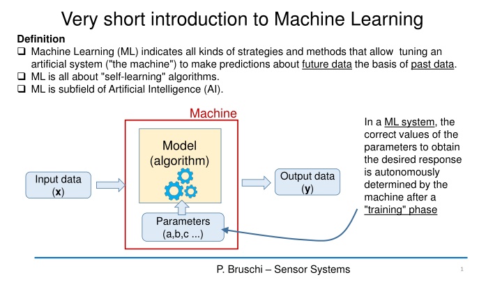
Very short introduction to Machine Learning Definition Machine Learning (ML) indicates all kinds of strategies and methods that allow tuning an artificial system ("the machine") to make predictions about future data the basis of past data. ML is all about "self-learning" algorithms. ML is subfield of Artificial Intelligence (AI). Machine In a ML system, the correct values of the parameters to obtain the desired response is autonomously determined by the machine after a "training" phase Model (algorithm) Output data (y) Input data (x) Parameters (a,b,c ...) P. Bruschi Sensor Systems 1

Example of Applications of Machine Learning Every kind of feature recognition in images (faces, objects, hazards, etc.) Voice recognition (form sounds to words) Text interpretation (spam filters, web-search tasks, document selection ...) Pattern recognition from homogeneous or heterogeneous sensor data (chemical component recognition, medical diagnosis, food quality ...) P. Bruschi Sensor Systems 2

The tree different cases of Machine Learning 1) Supervised learning 2) Unsupervised learning 3) Reinforcement learning P. Bruschi Sensor Systems 3

Supervised Learning Sometimes called "target" Single input data "example" Training: A large number of examples (labelled data) is proposed to the machine that learns to associate different labels (y) to different properties of the feature vector (x). x x 1 + Label y 2 ... x Goal: Tune the algorithm (i.e. its parameters) is such a way that it gets able to predict the label of all new x feature vector that are proposed to it after training. k Set of "features", or "predictors" that can be arranged into a row or column vector x Data in this format are called "labeled data" P. Bruschi Sensor Systems 4

Supervised Learning There are three main cases of supervised learning, depending on the type of label Binary (only two values, e.g. "yes / not") Binary classification Label Discrete (only a set of n possible values) Multi-class classification Regression Continuous (e.g. a real number) These categories are independent of the type of input data (i.e. type of features), which can be continuous even in the case of binary or discrete label P. Bruschi Sensor Systems 5

Unsupervised learning x x The goal of the training is finding hidden characteristics that can be used to find a criterion to classify the data (data clustering) or to eliminate useless information (dimensionality reduction) 1 2 ... x k Single input data "example" To illustrate the typical goals of unsupervised learning it is better to show a few examples. Data are "unlabeled" P. Bruschi Sensor Systems 6

Example of Data Clustering The clustering algorithm understand that data can be grouped into three "clusters". After clustering, a label can be created to signify belonging to a given cluster. x2 x x 1 2 x2 In this example the label can assume three values (red, green, blue) Feature vector x1 Graphical representation of the training set (27 examples) x1 Once we have learnt this property of the data (that we did not know before) we still have to give an interpretation to it and if it is useful, use this information to simplify classification algorithms. P. Bruschi Sensor Systems 7

Example of dimensionality reduction The dimensionality reduction task consists in finding coordinate transformation that allow reducing the number of significant features x2 x2 x1 x1 With this transformation, classification is much easier It is clearly possible to arrange data according their position in the spiral (coordinate z). We have a set of labelled data (green / red) with a 2-D vector. Depending on the algorithm, classificantion can be difficult with data arranged in this way. P. Bruschi Sensor Systems 8

Reinforcement learning Reinforcement algorithms learn how to perform actions in response to particular situations with the goal to obtain a certain result. Examples of goals are maximizing the profit of a company, winning a chess match etc .. Environment (set of states) Reward The algorithm learns which actions are convenient on the basis of the reward, which is a function of the state. The reward can be positive (win) or negative (loose). Training Agent (algorithm) action P. Bruschi Sensor Systems 9

Machine learning in sensor applications Machine learning can be used at this stage Digital Domain Analog domain Digital Processing Linear Filtering Data Interpretation Data compression Non-electrical sensor(s) AFE Analog Front-End ADCs Electrical probe(s) Display Communication Environment Storage P. Bruschi Sensor Systems 10

Machine learning in sensor applications Example: gas classification and/or concentration measurement y: concentration of the three gases (regression) x x x Machine Learning algorithm 1 Sensor 2 y 2 Sensor 3 3 y: type of gas or type of mixture (multi-class classification) Building of the feature vector P. Bruschi Sensor Systems 11

When is ML useful for data interpretation in sensors Data interpretation can be accomplished in two ways: 1. Model-driven: we know the deterministic relationship between the quantities that we want to sense and the sensor outputs ("features"). If the inverse relationship (from the features to the quantities) can be easily found, then it is directly implemented in the algorithm. 2. Data-driven: if the relationship between from the quantities to the sensor outputs is difficult-to-model, due to a large number of features, presence of strong non-linearities, unreliable properties, complicated dependencies, then its better to use a generic model and let the data tune it to perform the required data interpretation. Machine learning (= statistical learning) P. Bruschi Sensor Systems 12

General characteristics of the training process Hyperparameters: these are not parameter of the model (i.e. they do not affect the algorithm) but they may change: a) The structure of the model b) The way the training process is performed For example, in a polynomial regression process, an hyperparameter can be the degree of the polynomial. Cost or loss function: measure the difference between the desieed outputs and the predicted values y :predicted by the model 1 N N ( ) Example of loss function 2 y y i i = 1 i In all phases, proper cost functions are used to assess the degree of accuracy. P. Bruschi Sensor Systems 13

Data used in the training process Used to really train the algorithm (i.e. set the model parameters) Training data Used to choose the hyperparameters Development data Used at the end of the learning process to test the accuracy of the model Test data P. Bruschi Sensor Systems 14

Types of ML algorithms Decision trees (classification) Regression Analysis (regression, continuous target y) K-Nearest-Neighbors (k-NN) (classification) Logistic Regression (classification) Principal Component Analysis (PCA) (clustering) Artificial Neural Networks (ANN) (classification and /or regression) P. Bruschi Sensor Systems 15

Artificial Neural Networks: the origins The predecessor: The Perceptron (Ronsenblatt, Cornell Aerounautical Lab.1958) Originally implemented on a IBM 704 computer and connected to an array of photodetector to obtain a visual classifier. Inspired by: 1943: First models of the natural neuron (McCulloch-Pitt) Followed by: 1960: Adaline (ADAptive LInear NEuron) (B. Widraw et al., Stanford) P. Bruschi Sensor Systems 16

The perceptron classifier Inputs (features) x M w M D 1 1 = x w = x w = = x w , i i 1 i x w D D bias + + x w x w 1 0 0 if if b b = y 1 Parameters (weigths) P. Bruschi Sensor Systems 17

The perceptron operation: 2D case + + x w x w 1 0 0 if if b b = y 1 x w b x x 1 = x x2 x w b x2 y=1 w 2 w w w 1 = w x1 x x1 2 y=-1 = x w 0 constant = x w 0 constant P. Bruschi Sensor Systems 18

Perceptron classifier Training data Labels y (0 or 1) Target: find the correct weight set (w1, w2) and bias b that allow the perceptron to predict the label on a new data. In the case shown above, the data are "linearly separable", i.e. a line exists that divide the x1,x2plane into two regions where points with homogeneous label are present (1) 1 (1) 1 (3) 1 x (1) 2 (1) 2 (3) 2 x x x x x 1 1 1 ... 1 ..... ...... x ( ) ( 2 ) N N x 1 Since the plane exists, this classification problem can be solved by a perceptron The problem is: how to make the perceptron set the weights and the bias autonomously. P. Bruschi Sensor Systems 19

Setting the weights from the training data = learning Update algorithm ( ) + = + + y ( 1) + i: 1, .... D ( ) b n = b n y i i ( ) ( ) y x 1 ( ) w n w n y z i i i i i : learning rate D = z x w i i = 0 i ( ) ( ) + = + y x 1 ( ) w n w n y = = 1 w b x i i i i i 0 0 i: 0, .... D P. Bruschi Sensor Systems 20

Artificial Neural Networks The perceptron implements a "single layer" ANN and can solve only binary classification problems for linearly separable data An ANN uses more perceptrons (modified to produce a continuous output) to solve a much wider variety of problems P. Bruschi Sensor Systems 21