Introduction to Maximum Likelihood Estimation in Pattern Recognition

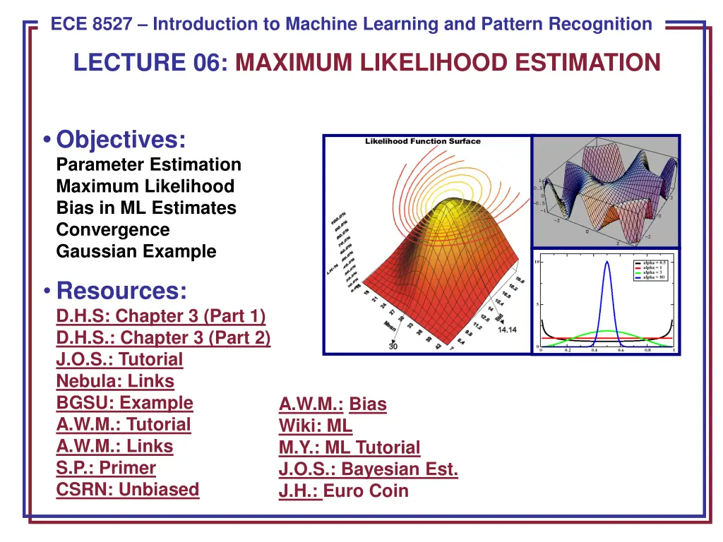
ECE 8443 Pattern Recognition ECE 8527 Introduction to Machine Learning and Pattern Recognition LECTURE 06: MAXIMUM LIKELIHOOD ESTIMATION Objectives: Parameter Estimation Maximum Likelihood Bias in ML Estimates Convergence Gaussian Example http://www.weibull.com/LifeDataWeb/image/apa_fig3.gif http://www.mat.ulaval.ca/informatique/guide94/img14.png Resources: D.H.S: Chapter 3 (Part 1) D.H.S.: Chapter 3 (Part 2) J.O.S.: Tutorial Nebula: Links BGSU: Example A.W.M.: Tutorial A.W.M.: Links S.P.: Primer CSRN: Unbiased A.W.M.: Bias Wiki: ML M.Y.: ML Tutorial J.O.S.: Bayesian Est. J.H.: Euro Coin

Introduction to Maximum Likelihood Estimation In Chapter 2, we learned how to design an optimal classifier if we knew the prior probabilities, P( i), and class-conditional densities, p(x| i). What can we do if we do not have this information? What limitations do we face? There are two common approaches to parameter estimation: maximum likelihood and Bayesian estimation. Maximum Likelihood: treat the parameters as quantities whose values are fixed but unknown. Bayes: treat the parameters as random variables having some known prior distribution. Observations of samples converts this to a posterior. Bayesian Learning: sharpen the a posteriori density causing it to peak near the true value. ECE 8527: Lecture 06, Slide 1

General Principle I.I.D.: c data sets, D1,...,Dc, where Djdrawn independently according to p(x| j). Assume p(x| j) has a known parametric form and is completely determined by the parameter vector j (e.g., p(x| j) ~ N( j, j), where j=[ 1, ..., j , 11, 12, ..., dd]). p(x| j) has an explicit dependence on j:p(x| j, j) Use training samples to estimate 1, 2,..., c Functional independence: assume Di gives no useful information about jfor i j. Simplifies notation to a set Dof training samples (x1,... xn) drawn independently from p(x| ) to estimate . Because the samples were drawn independently: n = x = k ( | ) ( ) p D p k 1 ECE 8527: Lecture 06, Slide 2

Example of ML Estimation p(D| ) is called the likelihood of with respect to the data. The value of that maximizes this likelihood, denoted , is the maximum likelihood estimate (ML) of . Given several training points Top: candidate source distributions are shown Which distribution is the ML estimate? Middle: an estimate of the likelihood of the data as a function of (the mean) Bottom: log likelihood ECE 8527: Lecture 06, Slide 3

General Mathematics t The ML estimate is found by solving this equation: = Let ( , ,..., ) . 1 2 p n ( ( ) ) 1 = x k [ ln 1 = ] l p = k Let . n ( ( ) ) = = k = x ln . 0 p p k 1 ( ) ( ) Define : ln l p D The solution to this equation can be a global maximum, a local maximum, or even an inflection point. Under what conditions is it a global maximum? ( ) = arg max l n = x = k ln( ( )) p k 1 n ( ( ) ) = x = k ln p k 1 ECE 8527: Lecture 06, Slide 4

Maximum A Posteriori Estimation ( ) ( ) p A class of estimators maximum a posteriori (MAP) maximize l where describes the prior probability of different parameter values. ( ) p An ML estimator is a MAP estimator for uniform priors. A MAP estimator finds the peak, or mode, of a posterior density. MAP estimators are not transformation invariant (if we perform a nonlinear transformation of the input data, the estimator is no longer optimum in the new space). This observation will be useful later in the course. ECE 8527: Lecture 06, Slide 5

Gaussian Case: Unknown Mean Consider the case where only the mean, = , is unknown: ( ) ( ) 0 ln 1 = k n = x p k 1 / 1 t 1 = x x x ln( ( )) ln[ exp[ ( ) ( )] p k k k / 1 2 2 d 2 2 ( ) 1 1 t 1 d = x x ln[( 2 ) ] ( ) ( ) k k 2 2 1 = xk x which implies: ln( ( )) ( ) p k 1 1 because: t 1 d x x [ ln[( 2 ) ] ( ) ( )] k k 2 2 1 1 t 1 d = x x [ ln[( 2 ) ] [ ( ) ( )] k k 2 2 1 = x ( ) k ECE 8527: Lecture 06, Slide 6

Gaussian Case: Unknown Mean Substituting into the expression for the total likelihood: n n ( ( ) ) 1 = = k = = x x = k ln ( ) 0 l p k k 1 1 n 1 ) = x = k ( 0 Rearranging terms: k 1 n ) = x = k ( 0 k 1 n n = x = k = k 0 k 1 1 n = x = k 0 n k 1 n 1 = x = k k n 1 Significance??? ECE 8527: Lecture 06, Slide 7

Gaussian Case: Unknown Mean and Variance Let = [ , 2]. The log likelihood of a SINGLE point is: 1 1 1 = t ln( ( )) ln[( 2 ) ] ( ) ) p x x (x k 2 1 2 1 k k 2 2 1 ( ) x 1 k 2 = = ln( ( )) l p x k 2 1 ( ) x 1 k + 2 2 2 2 2 The full likelihood leads to: n 1 = = k ( ) 0 x 1 k 1 2 2 n n n 1 ( ) x 2 1 k + = = = k = k = k 0 ( ) x 1 2 k 2 2 2 2 1 1 1 2 ECE 8527: Lecture 06, Slide 8

Gaussian Case: Unknown Mean and Variance n 1 n = = This leads to these equations: = k x 1 k 1 n 1 n 2 2 = = ) ( = k x 2 k 1 n 1 = In the multivariate case: x = n k n 1 1 k ( 1 )( ) t 2 = x x = k k k n ( )( )t x x The true covariance is the expected value of the matrix , which is a familiar result. k k ECE 8527: Lecture 06, Slide 9

Convergence of the Mean Does the maximum likelihood estimate of the variance converge to the true value of the variance? Let s start with a few simple results we will need later. Expected value of the ML estimate of the mean: n 1 2 2 ] = ] = = i [ [ ] E E x var[ [ ] ( [ ]) E E i n 1 2 2 = [ ] E n 1 = = n [ ] E x i n n 1 n 1 n n 1 2 1 i = = i = j [ ] E x x i j 1 1 = = = i n 2 1 = i n n 1 n 2 = [ ] E x x i j 2 = 1 1 j ECE 8527: Lecture 06, Slide 10

Variance of the ML Estimate of the Mean The expected value of xixj,, E[xixj,], will be 2 for i j and 2 + 2 otherwise since the two random variables are independent. The expected value of xi2 will be 2 + 2. Hence, in the summation above, we have n2-n terms with expected value 2 and n terms with expected value 2 + 2. Thus, ( ( ) ( ) ) 2 1 2 2 2 2 2 ] = + + = var[ n n n 2 n n which implies: 2 n 2 2 2 = ] + = + [ ] var[ ( [ ]) E E We see that the variance of the estimate goes to zero as n goes to infinity, and our estimate converges to the true estimate (error goes to zero). ECE 8527: Lecture 06, Slide 11

Variance Relationships We will need one more result: 2 2 2 2 = = + [( ) [ ] 2 [ ] [ ] E x E x E x E 2 2 2 = + [ ] 2 [ ] E x E 2 2 = [ ] E x n n 1 n 2 i 2 = = i = i ( ) x x i 1 1 Note that this implies: n ix 2 2 2 = + = i 1 Now we can combine these results. Recall our expression for the ML estimate of the variance: n 1 ( ) 2 2 = = i [ ] E ix n 1 ECE 8527: Lecture 06, Slide 12

Covariance Expansion Expand the covariance and simplify: n = n = 1 n n = 1 n ( ) 2 2 2 i 2 = = + [ [ ( 2 )] E x E x x i i 1 1 i i 1 n 2 i 2 = ] + ( [ ] 2 [ [ ]) E x E x E i 1 i n 1 n 2 2 2 2 = + ] + + (( 1 = ) 2 [ ( )) E x n i i One more intermediate term to derive: n = n = n = 1 1 ] = = = + [ [ ] [ ] ( [ ] [ ]) E x E x x E x x E x x E x x i i j i j i j i i n n 1 j 1 1 j j i j ( ) 2 1 1 2 2 2 2 2 2 = ) 1 + + = + = + (( ) (( ) n n n n n ECE 8527: Lecture 06, Slide 13

Biased Variance Estimate Substitute our previously derived expression for the second term: 1 n n = = + ] + + 2 2 2 2 2 (( ) 2 [ ( )) E x n i 1 i 1 n n = = + + + + 2 2 2 2 2 2 (( ) ( 2 ) ( )) n n 1 i 1 n n = = + + + 2 2 2 2 2 2 ( 2 2 ) n n 1 i 1 n n = = 2 2 ( ) n 1 i ) 1 1 n 1 n 1 n ( n n n n = = = = = / 1 = 2 2 2 2 ( ) 1 ( ) n n n 1 ) 1 n 1 1 i i i ( n = 2 ECE 8527: Lecture 06, Slide 14

Expectation Simplification Therefore, the ML estimate is biased: n 1 n n 1 n ( ) 2 2 2 2 = = [ ] E x = i 1 i However, the ML estimate converges (and is MSE). An unbiased estimator is: 1 n ( )( ) t = x C x = 1 i i 1 n i These are related by: n ) 1 ( = C n which is asymptotically unbiased. See Burl, AJWills and AWM for excellent examples and explanations of the details of this derivation. ECE 8527: Lecture 06, Slide 15

Summary To develop an optimal classifier, we need reliable estimates of the statistics of the features. In Maximum Likelihood (ML) estimation, we treat the parameters as having unknown but fixed values. Justified many well-known results for estimating parameters (e.g., computing the mean by summing the observations). Biased and unbiased estimators. Convergence of the mean and variance estimates. ECE 8527: Lecture 06, Slide 16