Introduction to Probability Theory and Experiments in Statistical Methods
Explore the fundamental concepts of probability theory and experiments in statistical methods, including classical examples like flipping coins and rolling dice. Understand the basics of events, outcomes, and uncertainty in research experiments. Gain insights into simple and compound outcomes, notation for event spaces, and more.

Download Presentation

Please find below an Image/Link to download the presentation.
The content on the website is provided AS IS for your information and personal use only. It may not be sold, licensed, or shared on other websites without obtaining consent from the author. If you encounter any issues during the download, it is possible that the publisher has removed the file from their server.
You are allowed to download the files provided on this website for personal or commercial use, subject to the condition that they are used lawfully. All files are the property of their respective owners.
The content on the website is provided AS IS for your information and personal use only. It may not be sold, licensed, or shared on other websites without obtaining consent from the author.
E N D
Presentation Transcript
Corpora and statistical methods Lecture 1, Part 2 Albert Gatt
In this part We begin with some basic probability theory: the concept of an experiment The concept of probability Rules of probability CSA5011 -- Corpora and Statistical Methods
The concept of an experiment and classical probability
Experiments The simplest conception of an experiment consists in: a set of events of interest possible outcomes simple: (e.g. probability of getting any of the six numbers when we throw a die) compound: (e.g. probability of getting an even number when we throw a die) uncertainty about the actual outcome This is a very simple conception. Research experiments are considerably more complex. Probability is primarily about uncertainty of outcomes. CSA5011 -- Corpora and Statistical Methods
The classic example: Flipping a coin We flip a fair coin. (our experiment ) What are the possible outcomes? Heads (H) or Tails (T) Either is equally likely What are the chances of getting H? One out of two P(H) = = 0.5 CSA5011 -- Corpora and Statistical Methods
Another example: compound outcome We roll a die. What are the chances of getting an even number? There are six possible outcomes from rolling a die, each with a 1 out of 6 chance There are 3 simple outcomes of interest making up the compound event of interest: even numbers: {2, 4, 6} any of these qualifies as success in our exp. effectively, we can be successful 3 times out of 6. P(Even) = 3/6 = 0.5 CSA5011 -- Corpora and Statistical Methods
Yet another example We write a random number generator, which generates numbers randomly between 0 and 200. Numbers can be decimals Valid outcomes: 0, 0.00002, 1.1, 4 NB: The set of possible outcomes is infinite uncountable (continuous) CSA5011 -- Corpora and Statistical Methods
Some notation We use to denote the total set of outcomes, our event space Can be infinite! (cf. the random number generator) discrete event space: events can be identified individually (throw of dice) continuous event space: events fall on a continuum (number generator) We view events and outcomes as sets CSA5011 -- Corpora and Statistical Methods
Venn diagram representation of the dice- throw example Possible outcomes: {1,2,3,4,5,6} Outcomes of interest (denoted A): {2,4,6} A 1 2 3 5 4 6 CSA5011 -- Corpora and Statistical Methods
Probability: classical interpretation Given n equally possible outcomes, and m events of interest, the probability that one of the m events occurs is m/n. If we call our set of events of interest A, then: Number of events of interest (A) over total number of events | | A = ( ) P A | | Principle of insufficient reason (Laplace): We should assume that events are equally likely, unless there is good reason to believe they are not. CSA5011 -- Corpora and Statistical Methods
Compound vs. simple events If A is a compound event, then P(A) is the sum of the probabilities of the simple events making it up: A a The sum of probabilities, for all elements a of A = ( ) ( ) P A P a Recall, that P(Even) = 3/6 = 0.5 In a throw of the Dice, the simple events are {1,2,3,4,5,6}, each with probability 1/6 P(Even) = P(2), P(4), P(6) = 1/6 * 3 = 0.5 CSA5011 -- Corpora and Statistical Methods
More rules Since, for any compound event A: a = ( ) ( ) P A P a A the probability of all events, P( ) is: e = = ( ) ( ) 1 P P e (this is the likelihood of anything happening , which is always 100% certain) CSA5011 -- Corpora and Statistical Methods
Yet more rules If A is any event, the probability that A does not occur is the probability of the complement of A: = ( ) 1 ( ) P A P A i.e. the likelihood that anything which is not in A happens. Impossible events are those which are not in . They have probability of 0. For any event A: ] 1 , 0 [ ( ) P A CSA5011 -- Corpora and Statistical Methods
Probability trees (I) Here s an even more complicated example: You flip a coin twice. Possible outcomes (order irrelevant): 2 heads (HH) 1 head, 1 tail (HT) 2 tails (TT) Only one way to obtain this: both throws give H Two different ways to obtain this: {throw1=H, throw2=T} OR {throw1=T, throw2=H} Only one way to obtain this: both throws give T Are they equally likely? No! CSA5011 -- Corpora and Statistical Methods
Probability trees (II) Four equally likely outcomes: outcome Flip 2 Flip 1 H HH 0.5 H 0.5 0.5 T HT 0.5 H TH 0.5 T 0.5 T TT CSA5011 -- Corpora and Statistical Methods
So the answer to our problem There are actually 4 equally likely outcomes when you flip a coin twice. HH, HT, TH, TT What s the probability of getting 2 heads? P(HH) = = 0.25 What s the probability of getting head and tail? P(HT OR TH) = 2/4 = 0.5 CSA5011 -- Corpora and Statistical Methods
Teaser: violations of Laplaces principle You randomly pick out a word from a corpus containing 1000 words of English text. Are the following equally likely: word will contain the letter e word will contain the letter h E is the most frequent letter in Engish orthography The is far more frequent than audacity What about: word will be audacity word will be the In both cases, prior knowledge or experience gives good reason for assuming unequal likelihood of outcomes. CSA5011 -- Corpora and Statistical Methods
Unequal likelihoods When the Laplace Principle is violated, how do we estimate probability? We often need to rely on prior experience. Example: In a big corpus, count the frequency of e and h Take a big corpus, count the frequency of audacity vs. the Use these estimates to predict the probability on a new 1000-word sample. CSA5011 -- Corpora and Statistical Methods
Example continued Suppose that, in a corpus of 1 million words: C(the) = 50,000 C(audacity) = 2 Based on frequency, we estimate probability of each outcome of interest: frequency / total P(the) = 50,000/1,000,000 = 0.05 P(audacity) = 2/1,000,000 = 0.000002 CSA5011 -- Corpora and Statistical Methods
Long run frequency interpretation of probability Given that a certain event of interest occurs m times in n identical situations, its probability is m/n. This is the core assumption in statistical NLP, where we estimate probabilities based on frequency in corpora. Stability of relative frequency: we tend to find that if n is large enough, the relative frequency of an event (m) is quite stable across samples In language, this may not be so straightforward: word frequency depends on text genre word frequencies tend to flatten out the larger your corpus (Zipf) CSA5011 -- Corpora and Statistical Methods
The addition rule You flip 2 coins. What s the probability that you get at least one head? The first intuition: P(H on first coin) + P(H on second coin) But: P(H) = 0.5 in each case, so the total P is 1. What s wrong? We re counting the probability of getting two heads twice! Possible outcomes: {HH, HT, TH, TT} The P(H) = 0.5 for the first coin includes the case where our outcome is HH. If we also assume P(H) = 0.5 for the second coin, this too includes the case where our outcome is HH. So, we count HH twice.
Venn diagram representation Set A represents outcomes where first coin = H. Set B represents outcomes where second coin = H A and B are our outcomes of interest. (TT is not in these sets) A A and B have a nonempty intersection, i.e. there is an event which is common to both. Both contain two outcomes, but the total unique outcomes is not 4, but 3. B HT HH TH TT
Some notation A B = events in A and events in B = events which are in both A and B ( = probability that something which is either in A OR B occurs ) P A B = probability that something which is in both A AND B occurs ) ( B A P A A B B HT HH TH TT
Addition rule To estimate probability of A OR B happening, we need to remove the probability of A AND B happening, to avoid double-counting events. = + ( ) ( ) ( ) ( ) P A B P A P B P A B In our case: P(A) = 2/4 P(B) = 2/4 P(A AND B) = P(A OR B) = 2/4 + 2/4 = = 0.75
Prior knowledge Sometimes, an estimation of the probability of something is affected by what is known. cf. the many linguistic examples in Jurafsky 2003. Example: Part-of-speech tagging Task: Assign a label indicating the grammatical category to every word in a corpus of running text. one of the classic tasks in statistical NLP
Part-of-speech tagging example Statistical POS taggers are first trained on data that has been previously annotated. Yields a language model. Language models vary based on the n-gram window: unigrams: probability based on tokens (a lexicon) E.g. input = the_DET tall_ADJ man_NN model represents the probability that the word man is a noun (NB: it could also be a verb) bigrams: probabilities across a span of 2 words input = the_DET tall_ADJ man_NN model represents the probability that a DET is followed by an adjective, adjective is followed by a noun, etc. Can also do trigrams, quadrigrams etc.
POS tagging continued Suppose we ve trained a tagger on annotated data. It has: a lexicon of unigrams: P(the=DET), P(man=NN), etc a bigram model P(DET is followed by ADJ), etc Assume we ve trained it on a large input sample. We now feed it a new phrase: the audacious alien Our tagger knows that the word the is a DET, but it s never seen the other words. It can: make a wild guess (not very useful!) estimate the probability that the is followed by an ADJ, and that an ADJ is followed by a NOUN
Prior knowledge revisited Given that I know that theis DET, what s the probability that the following word audacious is ADJ? This is very different from asking what s the probability that audacious is ADJ out of context. We have prior knowledge that DET has occurred. This can significantly change the estimate of the probability that audacious is ADJ. We therefore distinguish: prior probability: Na ve estimate based on long-run frequency posterior probability: probability estimate based on prior knowledge
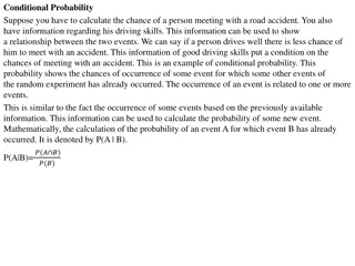
Conditional probability In our example, we were estimating: P(ADJ|DET) = probability of ADJ given DET P(NN|DET) = probability of NN given DET etc In general: the conditional probability P(A|B) is the probability that A occurs, given that we know that B has occurred
Example continued If I ve just seen a DET, what s the probability that my next word is an ADJ? Need to take into account: occurrences of ADJ in our training data VV+ADJ (was beautiful), PP+ADJ (with great concern), DET+ADJ etc occurrences of DET in our training corpus DET+N (the man), DET+V (the loving husband), DET+ADJ (the tall man)
Venn Diagram representation of the bigram training data A B is+tall the+man the+tall in+terrible a+simple the+woman an+excellent were+nice a+road Cases where w is ADJ NOT preceded by DET Cases where w is a DET followed by ADJ Cases where w is a DET NOT followed by ADJ
Estimation of conditional probability Intuition: P(A|B) is a ratio of the chances that both A and B happen, by the chances of B happening alone. ( ) P A B = ( | ) P A B ( ) P B P(ADJ|DET) = P(DET+ADJ) / P(DET)
Another example If we throw a die, what s the probability that the number we get is even, given that the number we get is larger than 4? works out as the probability of getting the number 6 P(even|>4) = P(even & >4)/P(>4) = (1/6) / (2/6) = = 0.5 Note the difference from simple, prior probability. Using only frequency, P(6)= 1/6
Multiplying probabilities Often, we re interested in switching the conditional probability estimate around. Suppose we know P(A|B) or P(B|A) We want to calculate P(A AND B) For both A and B to occur, they must occur in some sequence (first A occurs, then B)
Estimating P(A AND B) = ( ) ( ) ( | ) P A B P A P B A Probability that both A and B occur Probability of A Probability of B happening given that A has happened happening overall
Multiplication rule: example 1 We have a standard deck of 52 cards What s the probability of pulling out two aces in a row? NB Standard deck has 4 aces Let A1 stand for an ace on the first pick , A2 for an ace on the second pick We re interested in P(A1 AND A2)
Example 1 continued P(A1 AND A2) = P(A1)P(A2|A1) P(A1) = 4/52 (since there are 4 aces in a 52-card pack) If we do pick an ace on the first pick, then we diminish the odds of picking a second ace (there are now 3 aces left in a 51-card pack). P(A2|A1) = 3/51 Overall: P(A1 AND A2) = (4/52) (3/51) = .0045
Example 2 We randomly pick two words, w1 and w2, out of a tagged corpus. What are the chances that both words are adjectives? Let ADJ be the set of all adjectives in the corpus (tokens, not types) |ADJ| = total number of adjectives A1 = the event of picking out an ADJ on the first try A2 = the event of picking out an ADJ on second try P(A1 AND A2) is estimated in the same way as per the previous example: in the event of A1, the chances of A2 are diminished the multiplication rule takes this into account
Some observations In these examples, the two events are not independent of eachother occurrence of one affects likelihood of the other e.g. drawing an ace first diminishes the likelihood of drawing a second ace this is sampling without replacement if we put the ace back into the pack after we ve drawn it, then we have sampling with replacement In this case, the probability of one event doesn t affect the probability of the other.
Extending the multiplication rule The logic of the A AND B rule is: Both conditions, A and B have to be met A is met a fraction of the time B is met a fraction of the times that A is met Can be extended indefinitely E.g. chances of drawing 4 straight aces from a pack P(A1 & A2 & A3 & A4) = P(A1) P(A2|A1) P(A3|A1 & A2) P(A4|A1 & A2 & A3)
Extending the addition rule It s easy to extend the multiplication rule. Extending the addition rule isn t so easy. We need to correct for double-counting events. = + + ( ) ( P ) A ( B ) ( A ) P A B C P A P B P C ( ) ( ) ( ) P C P B C + ( ) P A B C
Example P(A OR B OR C) B A Once we ve discounted the 2-way intersection of A and B, etc, we need to recount the 3-way intersection! C
Subtraction rule Fundamental underlying observation: = ( ) 1 ( ) P A P A E.g. Probability of getting at least one head in 3 flips of a coin (a three-set addition problem) Can be estimated using the observation that: P(Head out of 3 flips) = 1-P(no heads) = 1-P(3 tails)
Switching conditional probabilities Problem 1: We know the probability that a test will give us positive in case a person has a disease. We want to know the probability that there is indeed a disease, given that the test says positive Useful for finding false positives Problem 2: We know the probability P(ADJ|DET) that some word w2 is an ADJ, given that the previous word w1 is a DET We find a new word w . We don t know its category. It might be a DET. We do know that the following word is an ADJ. We would therefore like to know the reverse , i.e. P(DET|ADJ)


")
")


")