Introduction to Reestimation and EM in Machine Learning

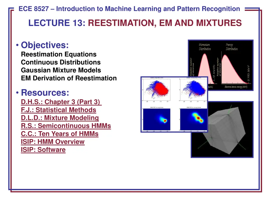
ECE 8443 Pattern Recognition ECE 8527 Introduction to Machine Learning and Pattern Recognition LECTURE 13: REESTIMATION, EM AND MIXTURES Objectives: Reestimation Equations Continuous Distributions Gaussian Mixture Models EM Derivation of Reestimation Resources: D.H.S.: Chapter 3 (Part 3) F.J.: Statistical Methods D.L.D.: Mixture Modeling R.S.: Semicontinuous HMMs C.C.: Ten Years of HMMs ISIP: HMM Overview ISIP: Software

Evaluation and Decoding (Review) ECE 8527: Lecture 13, Slide 1

Problem No. 3: Learning Let us derive the learning algorithm heuristically, and then formally derive it using the EM Theorem. Define a backward probability analogous to i(t): ( ) ( ) t = 0 t and t T 0 i ( ) t = = otherwise = 1 and t T 0 i i ( ) ( ) + + j 1 1 t a b v t j ij jk This represents the probability that we are in state i(t) and will generate the remainder of the target sequence from [t+1,T]. Define the probability of a transition from i(t-1) to i(t) given the model generated the entire training sequence, vT: ( ) ( ) ) ( P v v 1 t a b t ( ) t i ij jk j = ij T The expected number of transitions from i(t-1) to i(t) at any time is simply the sum of this over T: . ( ) = t 1 T ijt ECE 8527: Lecture 13, Slide 2

Problem No. 3: Learning (Cont.) T c ( ) ikt = t 1 The expected number of any transition from i(t) is: T ( ) t = t = 1 k ij 1 = a Therefore, a new estimate for the transition probability is: ij T c ( ) t = t 1 ik T = 1 k ( ) t = = T l jl We can similarly estimate the output probability density function: 1 t t b ( ) v v = k ij ( ) t = t 1 jl l The resulting reestimation algorithm is known as the Baum-Welch, or Forward Backward algorithm: Convergence is very quick, typically within three iterations for complex systems. Seeding the parameters with good initial guesses is very important. The forward backward principle is used in many algorithms. ECE 8527: Lecture 13, Slide 3

Continuous Probability Density Functions ( ) j bi The discrete HMM incorporates a discrete probability density function, captured in the matrix B, to describe the probability of outputting a symbol. j 0 1 2 3 6 4 5 Signal measurements, or feature vectors, are continuous-valued N-dimensional vectors. In order to use our discrete HMM technology, we must vector quantize (VQ) this data reduce the continuous-valued vectors to discrete values chosen from a set of M codebook vectors. Initially most HMMs were based on VQ front-ends. However, for the past 30 years, the continuous density model has become widely accepted. We can use a Gaussian mixture model to represent arbitrary distributions: ( ) = 2 2 1 m im M M 1 1 im 1 t v v ( v v ( v v = = where = m exp ) ) 1 b c c 1 i im im im im Note that this amounts to assigning a mean and covariance matrix for each mixture component. If we use a 39-dimensional feature vector, and 128 mixtures components per state, and thousands of states, we will experience a significant increase in complexity ECE 8527: Lecture 13, Slide 4

Continuous Probability Density Functions (Cont.) It is common to assume that the features are decorrelated and that the covariance matrix can be approximated as a diagonal matrix to reduce complexity. We refer to this as variance-weighting. Also, note that for a single mixture, the log of the output probability at each state becomes a Mahalanobis distance, which creates a nice connection between HMMs and PCA. In fact, HMMs can be viewed in some ways as a generalization of PCA. Write the joint probability of the data and the states given the model as: ( ( ) ( ) ( ) k t = = 1 1 1 ) T T M M M = 1 t v v ( v v ( v v = = , ) ) p a b a b c ( ) ( ) , 1 ( ) t ( )t t , 1 t t t t t t k t k t = 1 t = 1 k k 2 T This can be considered the sum of the product of all densities with all possible state sequences, , and all possible mixture components, K: ( ( ) ( ) ( ) ( )t t k t t k t t t c b a p , 1 ) t v v ( v v = , ) and ( v v ) ( v v ) t t = , p p ECE 8527: Lecture 13, Slide 5

Application of EM We can write the auxiliary function, Q, as: ( v v ) ( v v ) t t , p ( ) ( ) y t ( ( ) t ) t = = ( v v ) log log , Q P P y p , p t The log term has the expected decomposition: ( ( = = t 1 ) T T T t b v v ( v v + + = t = t log , ) p a c ) ( ) , 1 ( ) t ( ) t t t k t k t t 1 1 The auxiliary function has three components: ( ) ( ) c c M c M ( ) ( ) b = + + a c = i = j 1 = j 1 Q Q 1 Q Q a b c i jk jk i jk jk = = 1 1 k k The first term resembles the term we had for discrete distributions. The remaining two terms are new: ( ) T = ( ) t b t b v v ( v v = = = , ) ) ( , log ) Q p j k k b jk t jk t jk 1 t ( ) T = ( ) t t v v = = = , ) ) c ( , log Q p j k k c c jk t jk jk 1 t ECE 8527: Lecture 13, Slide 6

Reestimation Equations ( ) b Q Maximization of requires differentiation with respect to the , b jk jk jk parameters of the Gaussian: . This results in the following: jk T T t ) v v v v ( v v ) ) ) ) = t = t ( , j k ( , )( j k t t jk t jk 1 1 = = jk jk T T = t = t ) ( , ) j k ( , ) j k 1 1 ( k j , where the intermediate variable, , is computed as: ( ) v v T ( v v ) t = t ( ) ( ) i a c b j ( ) p t 1 t ij jk jk t = = , , p t j k k t 1 = = ( v v ) ( , ) j k t c = i ( ) i T 1 The mixture coefficients can be reestimated using a similar equation: T = t ( , ) j k 1 = c jk T M = t 1 ( , ) j k t = 1 k ECE 8527: Lecture 13, Slide 7

Case Study: Speech Recognition Input Speech Based on a noisy communication channel model in which the intended message is corrupted by a sequence of noisy models Bayesian approach is most common: ) | ( ) | ( A P Acoustic Front-end ( ) P A W P W = P W A ( ) Objective: minimize word error rate by maximizing P(W|A) Acoustic Models P(A/W) P(A|W): Acoustic Model P(W): Language Model P(A): Evidence (ignored) Language Model P(W) Search Acoustic models use hidden Markov models with Gaussian mixtures. P(W) is estimated using probabilistic N-gram models. Recognized Utterance Parameters can be trained using generative (ML) or discriminative (e.g., MMIE, MCE, or MPE) approaches. ECE 8527: Lecture 13, Slide 8

Case Study: Acoustic Modeling in Speech Recognition ECE 8527: Lecture 13, Slide 9

Case Study: Fingerspelling Recognition ECE 8527: Lecture 13, Slide 10

Case Study: Fingerspelling Recognition ECE 8527: Lecture 13, Slide 11

Summary Hidden Markov Model: a directed graph in which nodes, or states, represent output (emission) distributions and arcs represent transitions between these nodes. Emission distributions can be discrete or continuous. Continuous Density Hidden Markov Models (CDHMM): the most popular form of HMMs for many signal processing problems. Gaussian mixture distributions are commonly used (weighted sum of Gaussian pdfs). Subproblems: Practical implementations of HMMs require computationally efficient solutions to: Evaluation: computing the probability that we arrive in a state a time t and produce a particular observation at that state. Decoding: finding the path through the network with the highest likelihood (e.g., best path). Learning: estimating the parameters of the model from data. The EM algorithm plays an important role in learning because it proves the model will converge if trained iteratively. There are many generalizations of HMMs including Bayesian networks, deep belief networks and finite state automata. HMMs are very effective at modeling data that has a sequential structure. ECE 8527: Lecture 13, Slide 12