Inventory Management and Optimization Techniques for Operational Efficiency

Inventory Basic Model How can it be that mathematics, being after all a product of human thought which is independent of experience, is so admirably appropriate to the objects of reality? Albert Einstein

Why We are interested in reducing inventory Has carrying cost Physical carrying costs we need storage and human resources. Financial costs (Opportunity Cost) We could have invested our capital elsewhere and benefit from it. In the LFT Game financial cost is 10% of the cost of goods. Has Hidden Costs Devaluation Cost- Components typically drop in price during their inventory life Price Protection Cost. To reimburse customers for the drops in the prices. Return Cost Obsolescence Cost Hides problems Even if we produce low quality product, there is enough inventory downstream. Untrustworthy suppliers, machine breakdowns, long changeover times, scraps and defects do not show up. Long flow time, Feedback loop is long. not-uniform operations. Basic Inventory Problems. Models-Economies of scale 2

Impact of Changes- Not EOQ Monthly demand for a widget is 600 units; S= $100, C=$50, H= $9. Yearly demand is 7200 units. Assume a month is 30 days. Daily demand = 600/30 = 20 units per day. Compute EOQ EOQ= SQRT(2DS/H)= SQRT(2*7200*100/9) = 400 That is enough for how many days? # of days = 400/20 = 20 T? =?? 2 400 2 Suppose that widgets are packed in boxes of 500 25% increase in order quantity. Q= 500 =500/400= 1.25 = 25% more than EOQ TC= SD/Q+HQ/2 = 100(7200/500) + 9(500/2) TC = 1440 + 2250 = 3690 TC2/TC1= 3690/3600 = 2.5% Q 25% TC 2.5% ?+?? 7200 400 = 100 + 9 = 2??? = 2(100)(7200)(9) = 3600 Basic Inventory Problems. Models-Economies of scale 3

Impact of Changes in Demand on EOQ Suppose that the demand increases k=4 times. What is the change in the optimal order quantity, cycle stock, and # of orders per year? S=100, H=9, D1= 7200, D2=4(7200)=28800, EOQ1 = 400 EOQ1= SQRT(2*100*7200/9) = 400 EOQ2= SQRT(2*100*4(7200)/9) = 800 4D 2EOQ Demand is multiplied by K, EOQ is multiplied by SQRT(K) Basic Inventory Problems. Models-Economies of scale 4

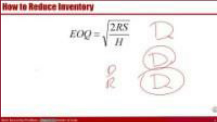
How to Reduce Inventory 2 RS = EOQ H To reduce EOQ we may R, S, H Two ways to reduce average inventory - Reduce S - Centralize S does not increase in proportion of Q EOQ increases as the square route of demand. - Commonality, modularization and standardization is another type of Centralization - Postponement, Delayed Differentiation Basic Inventory Problems. Models-Economies of scale 5

Reducing S JIT By considering fixed cost as a setup cost, EOQ can be used to determine optimal production size. Setup time reduction in just-in-time (JIT) production systems leads to smaller batches. Equipment with low set-up times Nearby suppliers with long-term relationships Uniform plant loading Low inventories with tight control Small batch and mixed-model production Basic Inventory Problems. Models-Economies of scale 6

Mixed Model Production Three products A, B, C. Production time: each 10 mins (Tp=10 mins). Plant is working 5 days a week, 10 hours a day. Demand at down stream station is A:3, B:2, C:1 units per hour. The upstream station in each production run produces one week of demand: A(150), B(100), and C(50). While the customer need it at hourly rates (either to consume or use it in production of another item) we ship it at weekly demand. Icycle = A(75), B(50), C(25). That is 150 What if we produce AAABBC. Then the Icycle is 3. An even better model is ABACBA Day Day Product A B C 1 2 3 0 4 0 5 0 6 0 7 0 0 8 0 0 9 0 0 10 0 0 100 400 Total 1000 800 Product A B C 1 2 3 0 4 0 5 0 6 7 0 8 0 0 9 0 10 0 0 100 400 Total 1000 800 500 0 0 500 0 0 500 0 0 0 500 200 0 200 0 200 0 200 0 200 0 0 200 0 0 200 200 0 100 100 100 100 0 100 0 0 100 Basic Inventory Problems. Models-Economies of scale 7

Setup Time Reduction- Toyota Production System Shigeo Shingo (Toyota) shortened setup times from several hours per each exchange of dies to a few minutes. He started by separating internal and external activities in a firm. Internal activities. Those for which it is essential for machine to be down such as (i) adjusting machine speed, (ii) placing work or fixtures on machine. Turn sequential internal activities into parallel activities or resources. Convert internal activities to external activities. External activities. Those for which it is not essential for machine to be down. Validating work order. Searching for tools and dies. Procuring material. External activities should be completed prior to setup. Standardize and practice setup routines to be perfect. Eliminate adjustments. Smooth and simplify procedures McLaren Applied Technologies team worked with GlaxoSmithKline to setup times in toothpaste production. Over six months changeover times dropped from 49 minutes to 15, translates into 7M more tubes of Sensodyne and Aquafresh a year Basic Inventory Problems. Models-Economies of scale 8

More Practice- The Next Few Slides are Not Recorded Basic Inventory Problems. Models-Economies of scale 9

Multiple Choice Questions 1. Most inventory models attempt to minimize A) the number of items ordered and the safety stock B) total inventory costs and likelihood of a stockout C) the number of orders placed and the average inventory D) All of the above E) None of the above 2. Inventory that is carried to provide a cushion against uncertainty of the demand is called A) Seasonal inventory B) Safety Stock C) Cycle stock D) Pipeline inventory E) Speculative inventory Basic Inventory Problems. Models-Economies of scale 10

Multiple Choice Questions 3. In the basic EOQ model, if annual demand doubles, the effect on the EOQ is: A) It doubles. B) It is four times its previous amount C) It is half its previous amount D) It is about 70% of its previous amount E) It increases by just above 40% 2 DS 2 ( 2 ) D S 1= EOQ 2 = EOQ H H 2 DS = . 1 = 2 2 41 1 EOQ EOQ H Basic Inventory Problems. Models-Economies of scale 11

S, H and R in the Game 60 kits in a product @ $10 / kit Input Material Cost = $600 Interest rate about 10% H = 10%(600) = $60/year 50 days + 7*24 days + 50 days = 268 days What is R? What is H? Estimate Average R for year, or for 268 days, or for month, or for day R /day H/365 = 60/365 = 16.5 cents/day R /month H/12 = 60/12 = $5/month R/268 day 268H/365 = Basic Inventory Problems. Models-Economies of scale 12

Why not Always Centralized If centralization reduces inventory, why doesn t everybody do it? Higher transportation cost Longer response time Less understanding of customer needs, cultural and regulatory barriers These disadvantages my reduce the demand. Basic Inventory Problems. Models-Economies of scale 13

Formula Proof for Total Cost of EOQ Total cost of any Q? TCQ = SR/Q + HQ/2 Total Cost of EOQ? The same as above, but can also be simplified 2?? ? 2 ? ?? + = ?????= 2?? ? 2?? ? 2 ? ?22?? ? 2?? ?= =? = 2??? ?????= 2 ?????= 2??? Basic Inventory Problems. Models-Economies of scale 14

Formula Proof for Flow Time Under EOQ Flow time when we order of any Q? Throughput = R, average inventory I = Q/2 RT = Q/2 T = Q/2R Flow time when we order of EOQ? Total Cost of EOQ? The same as above, but can also be simplified I = EOQ/2 2?? ? 2= ? =??? 2?? 4?= ?? 2? 2= T = I/R ?? 2? ?= ? ? = ?? 2??2 = ? T= 2?? Basic Inventory Problems. Models-Economies of scale 15

Multiple Choice Questions 1. The introduction of quantity discounts will cause the number of the units ordered to be: A) smaller than EOQ B) the same as EOQ C) greater than EOQ D) the same or smaller than EOQ E) the same or greater than EOQ Basic Inventory Problems. Models-Economies of scale 16