Inventory Optimization Strategies for LittleField Technologies

Order Quantity & Re-Order Point in LittleField Technologies Ardavan Asef-Vaziri

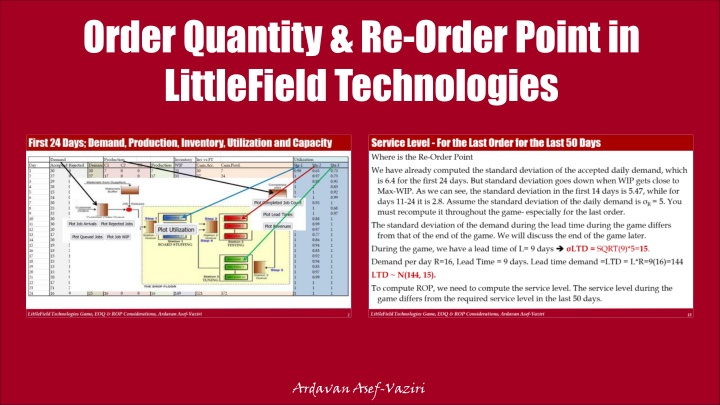
First 24 Days; Demand, Production, Inventory, Utilization and Capacity Demand Accepted Rejected 30 27 29 28 15 24 30 25 32 30 30 20 17 20 19 13 15 15 13 15 20 17 21 16 Production Inventory Inv vs FT Cum.Acc. 30 57 86 114 129 153 183 208 240 270 300 320 337 357 376 389 404 419 432 447 467 484 505 521 Utilization Sta-1 0.98 1 1 1 1 1 1 1 1 1 1 1 1 1 1 1 1 1 1 1 1 1 1 1 Day 1 2 3 4 5 6 7 8 9 10 11 12 13 14 15 16 17 18 19 20 21 22 23 24 DemandC1 30 27 29 28 15 24 30 25 32 30 30 20 17 20 24 35 32 20 25 24 29 17 23 25 C2 0 0 0 0 0 0 0 0 0 0 0 0 0 0 0 0 0 0 0 0 0 0 0 0 C3 0 0 0 0 0 0 0 0 0 0 0 0 0 0 0 0 0 0 0 0 0 0 0 0 Production WIP 7 17 15 17 17 17 15 20 14 14 20 14 10 14 15 13 15 16 13 16 19 20 18 16 Cum.Prod. 7 24 39 56 73 90 105 125 139 153 173 187 197 211 226 239 254 270 283 299 318 338 356 372 Sta-2 0.65 0.97 0.89 1 1 1 0.93 1 1 0.88 0.99 0.97 0.77 0.86 0.94 0.83 0.92 0.94 0.85 0.97 0.99 1 1 1 Sta-3 0.73 0.73 0.95 0.83 0.92 0.99 1 0.68 0.97 1 1 1 1 1 1 1 1 1 1 1 1 1 1 1 0 0 0 0 0 0 0 0 0 0 0 0 0 0 5 22 17 5 12 9 9 0 2 9 7 17 15 17 17 17 15 20 14 14 20 14 10 14 15 13 15 16 13 16 19 20 18 16 23 33 47 58 56 63 78 83 101 117 127 133 140 146 150 150 150 149 149 148 149 146 149 149 LittleField Technologies Game, EOQ & ROP Considerations, Ardavan Asef-Vaziri 2

The First 24 Days; Demand, Accepted Demand, Production, and Inventory LittleField Technologies Game, EOQ & ROP Considerations, Ardavan Asef-Vaziri 3

The First 24 Days; Demand, Accepted Demand, Production, and Inventory LittleField Technologies Game, EOQ & ROP Considerations, Ardavan Asef-Vaziri 4

Input, Output, Inventory, and Flow Time LittleField Technologies Game, EOQ & ROP Considerations, Ardavan Asef-Vaziri 5

Inventory Decisions in LittleField Technologies R and D are used interchangeably in our EOQ (Economic Order Quantity) models. D is Demand, and R is Throughput. We assume R = D Everything produced is sold. But when we do not allow all the Demand (arrival) to come in (due to a Max-WIP), then instead of Demand, we refer to Accepted Demand. For the first 24 days, the average output was 15.5. We assume R = D = 16 for the rest of the game until we increase the capacity. We assume the Demand is relatively stable at this level. We can later revise the Demand based on the new data. We need 60 kits for each contract at $10 per kit. While the Demand is probabilistic and moves up and down around the average, to be able to use the EOQ model, we need to assume that the Demand is deterministic. Therebefore, the kits are used at a steady rate per day, and a year is 365 days. The game assumes no storage and no obsolescence cost during the period that we have access to the game. The physical holding cost is 10% of the purchase price. We also have a 10% Capital Cost. The ordering cost is $1000 per order. How much should we order each time to minimize our total costs (total ordering and carrying costs)? LittleField Technologies Game, EOQ & ROP Considerations, Ardavan Asef-Vaziri 6

Inventry Profiles, Good & Bad Decisions LittleField Technologies Game, EOQ & ROP Considerations, Ardavan Asef-Vaziri 7

Number of Orders & Ordering Costs D = R = (16)(365) = 5840 contracts per year or D = R = 60(5840) = 350400 kits per year. H = 0.2($10) = $2 per kit per year, or H = $10*0.20(60) = $120 per contract per year. S = $1000 per order. Ordering Quantity = Q # of orders per year = D/Q = 5840/Q Ordering Cost per year = 1000(5840)/Q OC = SD/Q = 1000(5480)/2 LittleField Technologies Game, EOQ & ROP Considerations, Ardavan Asef-Vaziri 8

Average Inventory & Carrying Cost At the start of cycle, we have the order size Q units, at the end of the cycle we have 0. Average inventory = (Q+0)/2 = Q/2 units Q/2 is also called cycle inventory. Quantity Time In each cycle, we have Q/2 inventory In all cycles, we have Q/2 inventory. Throughout the year, we have Q/2 inventory. Cost of carrying (holding) one unit of inventory for one year = H $ per unit per year. Total Holding Costs (Total Carrying Costs) = CC = HQ/2 $ per year LittleField Technologies Game, EOQ & ROP Considerations, Ardavan Asef-Vaziri 9

Inventory Decisions in in LittleField Technologies CC = HQ/2 = 120Q/2 LittleField Technologies Game, EOQ & ROP Considerations, Ardavan Asef-Vaziri 10

Inventory Decisions in in LittleField Technologies LittleField Technologies Game, EOQ & ROP Considerations, Ardavan Asef-Vaziri 11

Economic Order Quantity At EOQ (Economic Order Quantity), OC = CC SD/Q = HQ/2 1000(5840)/Q = 120Q/2 Q2 = 97333.33 Q = 312 contracts SD/Q = HQ/2 Q2 = 2DS/H 2?? ? 2(5840)(1000) 120 = 312 ??? = ??? = That is one way to compute EOQ and not to memorize it. EOQ = 312(60) = 18720 kits Kits for 312 contracts are enough for how many days. 312/16 = 19.5 days. To find D, we did 16(365) = 5840, but the game only runs for 50+7(24)+50 = 50+168+50 = 268 days. Is our computation incorrect? It does not matter. Since $120 is the cost of carrying 60 kits for 365 days, for a demand of 268 days, $120 will be multiplied by 268/365, leading to H= $120(268/365) = 88.11. To clarify, let's use monthly demand instead of yearly demand. LittleField Technologies Game, EOQ & ROP Considerations, Ardavan Asef-Vaziri 12

Economic Order Quantity Since yearly demand is 5840, then monthly demand is 5840/12 = 486.6667. The ordering cost remains $1000 per order. The carrying cost is $120 for carrying 60 kits for one contract per year. Therefore, it is $120/12= $10 per month. 2(486.6667)(1000) 10 2?? ? = 311.9829 312 ??? = = The same is true for daily demand. We can have D=R=16 per day. S=$1000 per order, and H =120/365 = $0.328767123287671 2?? ? 2(16)(1000) 0.328767123287671 312 ??? = = Aslong as D and H are defined over the same period, year, month, week, and day, they all result in the same EOQ. The ordering cost is still S(D/Q), and the carrying cost is still H(Q/2). Nevertheless, throughout the game, based on the volume of demand and how you manage the capacity, you may use a different value as your yearly, or monthly demand (throughput) estimate each time. LittleField Technologies Game, EOQ & ROP Considerations, Ardavan Asef-Vaziri 13

Ordering Cost, Carrying Cost, Ordering Cycle, Flow Time, InvTurns OC= SD/Q = 1000(5840)/311.9829= 18718.97 CC = HQ/2 = 120(311.9829)/2 = 18718.97 Ordering Cycle = 312/16= 19.5 days Cycle Inventory = 312/2= 156 For the time being we assume the safety stock is 0 Therefore, average inventory is equal to cycle inventory I = Q/2 = 156 Flow time RT=I R=16 per day, I = 156 T= 156/16 = 9.75 Alternatively, (29.5+0)/2 = 9.75 days Inventory turns = R/I = 5840/156= 37.44 times InvTurns = 1/FlowTime =1/9.75 1/9.75 OR 37.44? 365(1/9.75) = 37.44 LittleField Technologies Game, EOQ & ROP Considerations, Ardavan Asef-Vaziri 14

Service Level - For the Last Order for the Last 50 Days Where is the Re-Order Point We have already computed the standard deviation of the accepted daily demand, which is 6.4 for the first 24 days. But standard deviation goes down when WIP gets close to Max-WIP. As we can see, the standard deviation in the first 14 days is 5.47, while for days 11-24 it is 2.8. Assume the standard deviation of the daily demand is R = 5. You must recompute it throughout the game- especially for the last order. The standard deviation of the demand during the lead time during the game differs from that of the end of the game. We will discuss the end of the game later. During the game, we have a lead time of L= 9 days LTD = SQRT(9)*5=15. Demand per day R=16, Lead Time = 9 days. Lead time demand =LTD = L*R=9(16)=144 LTD ~ N(144, 15). To compute ROP, we need to compute the service level. The service level during the game differs from the required service level in the last 50 days. LittleField Technologies Game, EOQ & ROP Considerations, Ardavan Asef-Vaziri 15

CSL For Continuously Stocked Item With & Without Lost Sales HQ DCu D=R per Y Days/Y D=R per d S/order H per unit per contract EOQ Cu Interest over 9 days 5840 365 16 1000 120 312 CSL* (Without Lost Sale) = 1 HQ CSL* (With Lost Sale) = 1 0.986301 0.993589 DCu+HQ LittleField Technologies Game, EOQ & ROP Considerations, Ardavan Asef-Vaziri 16

ROP - When We have Access to the Game We first discuss the service level at the end of the game. Suppose we are on a $1000 contract. What service level should we choose? What is the underage cost (Cu)? If a contract is available but cannot deliver it, we don t earn $1000. We would have spent $600 on the 60 kits required for each contract. Cu=$1000-$600=$400. However, we do not lose this profit because we earn it in the next cycle. Since each cycle is 19.5 20 days), the interest rate we do not earn is 10%. Therefore, underage cost Cu = 0.1(20/365)(400) = 2.2. What is the overage cost (Co)? If we order kits for one extra contract and do not use it in this cycle, we use them in the next cycle. But we have 20% financial and storage cost per carrying the 60 kits ($600) of a contract for one year. Therefore, average cost Co = 0.2(20/365)(600) = 6.6 SL* = 2.2/(2.2+6.6) = 0.25 LittleField Technologies Game, EOQ & ROP Considerations, Ardavan Asef-Vaziri 17

Service Level - For the Last Order for the Last 50 Days NORM.S.INV(0.25) = -0.67 standard deviation of lead time demand to the right. That is 0.67 to the left. We have already assumed the standard deviation of daily demand. Suppose it is R = 5. The standard deviation of the demand during the lead time during the game differs from that of the end of the game. During the game, we have a lead time of 9 days. Therefore, LTD = SQRT(9)*5=15. Is = -0.67 (15)=-10. Demand per day R=16, Lead Time = 9 days. Lead time demand =LTD = L*R=9(16)=144 LTD ~ N(144, 15). ROP=144-10=134 orders ROP = 176 orders x 60 kits/order = 10560 kits. We place an order Q= 18720 kits when inventory reaches ROP=10560 kits. But we have ignored a critical component in Cu. We did not discuss it since it needs knowledge beyond the mathematical content of our course. But we need to take it into account. LittleField Technologies Game, EOQ & ROP Considerations, Ardavan Asef-Vaziri 18

Service Level - For the Last Order for the Last 50 Days What if a shortage of kits leads to a delay in the contract delivery. A delay may reduce the revenue of a contract from 1000 to 0. That is a massive increase in Cu. Therefore, throughout the game, but not in the very last 50 days, apply a significant service level, say 3 standard deviations to the right- which is about %99 service level. Then monitor the inventory level. If you think you carry extra inventory instead of three standard deviations, you may choose two or even one standard deviation. But the situation is entirely different in the very last 50 days of the game. We place an order Q= 18720 kits when inventory reaches the kits required for 144+3*15 orders. That is 60(189)= 11340 kits. LittleField Technologies Game, EOQ & ROP Considerations, Ardavan Asef-Vaziri 19

The Last 50 Days; Inventory LittleField Technologies Game, EOQ & ROP Considerations, Ardavan Asef-Vaziri 20

Service Level - For the Last Order for the Last 50 Days What is L and what is LTD a few hours before when we will be disabled of making any changes. Suppose it is a little before 8 PM a day before the end of the game. The 218 days of the game ends at 1 PM tomorrow. The game then runs for 50 more days, but it takes a second for computer to do all the computations. Therefore, at 1:01 PM you can see your final standing. Now it is a little before 8 PM the day before, and we have 17 hours (days) to the last 50 days. Therefore, the game has 50+17 days to run. L=67. Demand per day = R=16 Demand in 67 days =LTD = L*R = 67(16) = 1072 Standard deviation of daily demand = R=5 Standard deviation of demand for 67 days of demand = LTD= SQRT(67)*5 40.9 41 LTD=N~(1072, 41) What are Cu and Co? LittleField Technologies Game, EOQ & ROP Considerations, Ardavan Asef-Vaziri 21

Service Level - For the Last Order for the Last 50 Days If a contract is there but the kits are not, you could have spent $600 and have earned $1000. Cu = $400. If kits for a contract are there but contract is not, you have no use for them, and at the end of the game their value is 0. Cu = $600. SL*=$400/($400+600) = 0.4 NORM.S.INV(0.396739) = -0.253standard deviation of lead time demand to the right. That is -0.253347103 to the left Is = -0.253347103 (41)=-10.38 -10 LTD=N~(1072, 41) Q= 1072-10= 1062 LittleField Technologies Game, EOQ & ROP Considerations, Ardavan Asef-Vaziri 22

Service Level - For the Last Order for the Last 50 Days Should we order the kits required for 1062 contracts? Should we order 63720 kits? No. Why We need to check how much inventory we have. Suppose we have 6000 kits which is enough for 100 contracts. Set your new order quantity 63720-6000= 57720 kits, then quickly set your ROP to more than 6000 kits to make sure that you trigger that materials order immediately. LittleField Technologies Game, EOQ & ROP Considerations, Ardavan Asef-Vaziri 23