Inverse Laplace Transform Tutorial and Differential Equations Solving

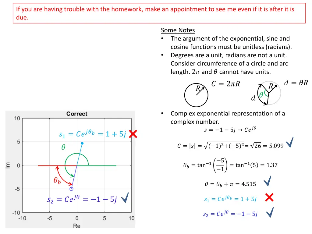
If you are having trouble with the homework, make an appointment to see me even if it is after it is due. Some Notes The argument of the exponential, sine and cosine functions must be unitless (radians). Degrees are a unit, radians are not a unit. Consider circumference of a circle and arc length. 2? and ? cannot have units. ? = ?? ? = 2?? ? ? ? ? Complex exponential representation of a complex number. ? = 1 5? ???? ?1= ?????= 1 + 5? ( 1)2+( 5)2= ? = ? = 26 = 5.099 ? ??= tan 1 5 = tan 15 = 1.37 1 ?? ? = ??+ ? = 4.515 ?2= ????= 1 5? ?1= ?????= 1 + 5? ?2= ????= 1 5?

Homework 2, Inverse Laplace Transform Node You may skip this example. The answers on this do not count in your grade.

In Lecture 2, we finished Laplace transforms. Today we will cover the inverse Laplace transform. Module 1 Goal: Use Laplace transforms to solve differential equations. Lecture 3 Inverse Laplace Transforms IVT and FVT Apply Laplace Transform to first and second order linear ordinary differential equations First Order Example Lecture 2 Inverse Laplace Transfrom The Laplace transform of the time derivative of a function ( ?(?)) was determined using integration by parts DerivativeInitial Condition Constant ? ?(?) = ?? ? ?(0) ? ? + ?? = ?? ?(?) Suppose we define ? ? to be ?(?), then ?? ??(0) ?? + ? ? ?(?) = ?? ? ?(0) ? ? = ? ?? + ? First Degree Polynomial Now since ? ? = ? ?(?) , we have Zero Root Second order ? ?(?) = ? ?(?) = ? ?? ? ?(0) ?(0) Derivatives Initial Conditions ? ? + ? ? + ?? = 0 ? ? =??? 0 + ? ? 0 + ??(0) ??2+ ?? + ? Second Degree Polynomial First Degree Polynomial ? ?(?) = ?2? ? ?? 0 ?(0) A dot becomes and ? Now we can use this for differential equations General form determines ? 1? ? and ? 1? ? to obtain ? ? and ? ? Methods to invert first and second order Laplace transforms Solving Differential Equations with Laplace Transforms Solving first order differential equations with Laplace transforms Solving second order differential equations with Laplace transforms (repeated real roots case) Identifying the graph of the response associated with a differential equation from the Laplace transform

So far, we have reviewed Laplace of a few basic functions: ? ?(?) =1 ?, 1 ? ? ??= ? + ?, ?2 ? sin ?? = ?2+ ?2 The Laplace transform of the time derivative of a function ( ?(?)) was determined using integration by parts ? ?(?) = ?? ? ?(0) ? ?(?) = ?2? ? ?? 0 ?(0)

So far, we reviewed Initial Value Theorem: If the function ?(?) is bounded and lim ? 0? ? exists, then the following is true. lim ? 0? ? = lim ? ??(?) This provides information about the starting point of a time domain function ?(?) from its Laplace representation ? ? . Final Value Theorem: If the function ?(?) is bounded and lim ? ? ? exists, then the following is true. lim ? ? ? = lim ? 0??(?) This provides information about the ending point of a time domain function ?(?) from its Laplace representation ? ? . ?? Final Value Theorem Initial Value Theorem ? 0 = lim ? 0? ? = lim ???= lim ? ? = ) ?(?? + ? ? ??(?) = lim =?? ? ? ??(?) ?? ?? + ? ? ? = lim ? 0??(?) ?? ?? = lim ? = lim ? ? = lim ? = 0 ) ) ?(?? + ? ?(?? + ? ? 0

Today, we will review Using partial Fraction Expansion to simplify a Laplace representation so that an Inverse Laplace operation can be implemented. Second-order system First-order system ? ? + ?? = ?? ?(?) ? ? + ? ? + ?? = 0 ? ? =??? 0 + ? ? 0 + ??(0) ??2+ ?? + ? ?? ??(0) ?? + ? ? ? = ? ?? + ?

The Laplace transform is applied to linear ODEs, the solution is obtained algebraically in the Laplace domain and then the time domain solution is obtained with the inverse Laplace transform. First Order Linear ODEs Lead to Laplace Functions of the Following Form Use Entry 6 ?0 =?0 1 ? ? = ?1? + ?0 ?1 ? + ?0/?1 Second Order Linear ODEs Lead to Laplace Functions of the Following Form ?1? + ?0 ?2?2+ ?1? + ?0 =?(?) ?(?) ? ? = The Roots of the denominator polynomial ? ? = ?2?2+ ?1? + ?0 determine the most efficient method to invert the Laplace transform and the form of the solution (oscillatory or exponential).

Step 1: Factor out the 4 in the numerator and the 11 in the denominator. 4 4 1 ? ? = 11? + 44= 11 ? + 4 Step 2: Use linearity of the inverse Laplace transform. 4 1 4 1 ? ? = ? 1 11? 1 = 11 ? + 4 ? + 4 Step 3: Use table entry 6 in the Laplace transform table. 4 11? 4? ? ? = 4 4 11 1 Comment: Suppose ? ? = 11? 44= ? 4. The solution is UNBOUNDED. 4 11?+4? x ? = 4 4 11 1 Comment: Suppose ? ? = ? 11?+44= . Use table entry ? ?+4 1 111 ? 4? ? ? =

For second order denominator polynomials ?(?), the roots of the denominator polynomial determine the form of the inverse transform. Second Order Problem ?1? + ?2 ?1?2+ ?2? +?3 The denominator polynomial is ? ? = ?1?2+ ?2? +?3. There are three possibilities. Real Distinct Roots ?1,2= ?, ?. Partial fractions expansion and entry 6. ? ? = ?1?+?2 ?1?2+?2?+?3= ?1 ?1 ?+?2/?1 (?+?)(?+?) ?1 ?+?+ ?2 ?+? ? ? = = Real Repeated Roots ?1,2= ?, ?. Partial fractions expansion and entries 6 and 7. ?1?+?2 ?1?2+?2?+?3= ?1 ?1 ?+?2/?1 (?+?)2 ?1 ?+?+ ?2 ? ? = = ?+?2 Complex Roots ?1,2= ? ??. Complete the square and use entries 20 and 21. ?1?+?2 ?1?2+?2?+?3= ?1 ?1 ?+?2/?1 (?+?)2+?2 ? ? =

Step 1: Factor out the 12 in the numerator and the 18 in the denominator. ? +1 18?2+ 324? + 1170=2 12? + 3 4 ? ? = ?2+ 18? + 65 3 Step 2: Find the roots of the denominator. ?2+ 18? + 65 = 0 182 4(1)(65) 2(1) ?1,2= 18 = 18 324 260 2(1) ?1,2= 18 64 = 18 8 2(1) = 5, 13 2(1) Step 3: Factor and complete a partial fractions expansion. ? + 1/4 ?2+ 18? + 65= ? + 1/4 ?1 ?2 (? + 5)(? + 13)= ? + 5+ ? + 13 Step 4: Find ?1 and ?2 by multiplying through by the denominator and strategically choosing values for s. lim ? 5? + 1/4 = ?1(? + 13) + ?2(? + 5) 19 ? 13? + 1/4 = ?1(? + 13) + ?2(? + 5) 51 4= ?1(8) ?1= 19 32 ? + 1/4 = ?1(? + 13) + ?2(? + 5) 4= ?2( 8) ?2=51 lim 32 Note that since ? is a variable, the values of ?1 and ?2 must be consistent with any values of ?. Thus we can choose ? to aid in finding ?1 and ?2.

Step 5: Put in ?1 and ?2. ? ? =2 3 ?2+ 18? + 65 ? + 1/4 ?(?) =2 19 32 1 +51 32 1 3 ? + 5 ? + 13 ?(?) = 19 1 +51 48 1 48 ? + 5 ? + 13 Step 6: Apply table entry 6 to both terms and simplify 51/48 to 17/16. ?(?) = 19 1 +17 16 1 48 ? + 5 ? + 13 ?(?) = 19 48? 5?+17 16? 13? Enter the answers in fractional form. We have worked to be sure that these all come out with even numbers and relatively simple fractions. Real roots of ? ? lead to and exponential, non-oscillatory time domain function. This behavior will be called overdamped.

Step 1: Factor out the 7 in the numerator and the 9 in the denominator. 9?2+ 18? + 909=7 7? + 7 ? + 1 ? ? = ?2+ 2? + 101 9 Step 2: Find the roots of the denominator. ?2+ 2? + 101 = 0 22 4(1)(101) 2(1) = 2 20? ?1,2= 2 = 2 4 404 2(1) ?1,2= 2 400 = 1 10? 2(1) 2(1) Step 3: Complete the square in the denominator. ? ? =7 ? + 1 =7 ? + 1 =7 ? + 1 ?2+ 2? + 1 1 + 101 ? + 12+ 100 ? + 12+ 102 9 9 9 Step 4: Use table entry 21. ? ? =7 ? + 1 ? + 12+ 102 9 ? ? =7 9? ?cos 10? Complex roots of ? ? lead to a decaying oscillatory time domain function. This behavior will be called underdamped.

For second order denominator polynomials ?(?), the roots of the denominator polynomial determine the form of the inverse transform. Second Order Problem ?1? + ?2 ?1?2+ ?2? +?3 =?(?) ?(?) ? ? = The denominator polynomial is ? ? = ?1?2+ ?2? +?3. There are three possibilities. Real Distinct Roots ?1,2= ?, ?. Partial fractions expansion and entry 6. ? ? = ?1?2+?2?+?3= ?1 (?+?)(?+?) Real Repeated Roots ?1,2= ?, ?. Partial fractions expansion and entries 6 and 7. ? ? = ?1?2+?2?+?3= ?1 (?+?)2 Complex Roots ?1,2= ? ??. Complete the square and use entries 20 and 21. ? ? = ?1?2+?2?+?3= ?1 ?1?+?2 ?1 ?+?2/?1 ?1 ?+?+ ?2 ?+? = Partial Fractions ?1?+?2 ?1 ?+?2/?1 ?1 ?+?+ ?2 = Partial Fractions ?+?2 ?1?+?2 ?1 ?+?2/?1 (?+?)2+?2 Complete Square Fourth Common Possibility: Third order case (step input) ?1?+?2 ? ?1?2+?2?+?3=?1 ?2?+?3 ?1?2+?2?+?3 ? ? = ?+ Treat this as above

Step 1: Factor out the 2 in the numerator and the 8 in the denominator. 2 ? 8?2+ 64? + 200 =1 4 ? ?2+ 8? + 25 Step 2: Use an alternate partial fractions expansion. 1 ? ?2+ 8? + 25 ? ? = 1 =?1 ?2? + ?3 ?2+ 8? + 25 ?+ Step 3: Multiply by the denominator. 1 = ?1?2+ 8? + 25 + ?2?2+ ?3? Step 4: Group terms with like powers of ?. 1 = ?1?2+ 8?1? + 25?1+ ?2?2+ ?3? 0 = ?1+ ?2?2+ 8?1+ ?3? + 25?1 1 ?0 Step 5: Recognize that the coefficient of each power of ? must be zero. ?1+ ?2= 0 ?2= ?1 ?2= 1 25 25?1 1 = 0 25?1= 1 8?1+ ?3= 0 ?3= 8?1 ?3= 8 1 ?1= 25 25

Step 6: Write the expansion. ? ? =1 4 ? ?2+ 8? + 25 1 ? ? =1 1 1 ? 1 ? + 8 ?2+ 8? + 25 4 25 25 Step 7: Find the roots of the denominator of the second term. ?2+ 8? + 25 = 0 82 4(1)(25) 2(1) ?1,2= 8 = 8 36 2(1) = 4 3? Step 8: Complete the square in the second term and break up to match entries 20 and 21. 1 1 ? ? + 4 + 4 ? + 42+ 32 1 100 1 100 ? + 8 1 1 ? ? + 8 ? + 42+ 9 ? ? = = ?2+ 8? + 16 16 + 25 100 1 ? 100 ? + 4 1 1 1 ? ? + 42+ 32 1 4(3) ? ? = = ? + 42+ 32 100 100 3 ? ? ? 4?cos 3? 4 9? 4?sin 3? 3? 4?sin 3? ? ? = 1 ? 4?cos 3? 4 ? ? =

The main points of Lecture 3 are given. Goal: Use Laplace transforms to solve linear first and second order ordinary differential equations. The Laplace transform allows a differential equation in the time domain to be interpreted as algebraic equations in the Laplace domain. The Laplace transform of the time derivative of a function naturally leads to solutions in the Laplace domain that consist of ratios of polynomials in ?. First order linear ODEs ?0 ?1? + ?0 Second order linear ODEs ?1? + ?2 ?1?2+ ?2? +?3 =?(?) ?(?) ? ? = ? ? = The inverse Laplace transform allows the Laplace domain functions to be written in the time domain. The roots of the denominator of the Laplace domain function determine the most efficient way to invert the Laplace transform and more importantly determines the mathematical behavior of the response. If the roots have negative real part, the solution will be bounded. First order linear ODEs lead with no sustained input lead to exponential solutions only. Second order linear ODEs can lead to exponential or damped exponential solutions. Distinct real roots exponential, non-oscillatory, overdamped (? ??) Repeated real roots exponential, non-oscillatory, critically damped (? ??, ?? ??) Complex roots damped sinusoidal, oscillatory, underdamped (? ??sin ?? , ? ??cos ?? )

Partial Fraction Expansion When using Laplace to solve LTI ODEs, the solution to the ODE in the Laplace domain is a ratio of polynomials in s. Let ? = ?(?)/? ? where ? ? and ? ? are polynomials in ?. Partial fraction expansion helps to solve for 1 { ( )} q s = L ( ) q t We write 1 m m + + + + ( ) ( ) N s N s N s N N s D s = = 1 n 1 + 0 m s m ( ) q s 1 n + + + D s D s s D 1 )( s 1 0 n z ( ) ( s ) N s s z z = 1 2 ) m s m ( )( ( ) p p p 1 2 n where ?? and ?? are complex numbers.

The main points of Lecture 2 are given. Goal: Use Laplace transforms to solve linear first and second order ordinary differential equations. Laplace transform tables summarize the Laplace transform of many common functions. The properties of Laplace transforms used in conjunction with the tables allow us to find the Laplace transforms of many other functions. For this course, the Laplace transform table it sufficient to all that we do. The Initial Value Theorem (IVT) and Final Value Theorem (FVT) allow us to deduce the behavior of a time domain function ? ? from its Laplace domain representation ?(?). The Laplace transform of the time derivative of a function naturally leads to solutions in the Laplace domain that consist of ratios of polynomials in ?. First order linear ODEs Second order linear ODEs ?0 ?1? + ?2 ?1?2+ ?2? +?3 =?(?) ?(?) ? ? = ? ? = ?1? + ?0 First order systems lead to exponential solutions. Second order systems lead to exponential solutions if the roots of ?(?) are real and distinct and lead to exponentially decaying oscillatory solutions if the roots of ?(?) are complex.

Some notes 1 m m + + + + ( ) ( ) N s N s N s N N s D s = = 1 n 1 + 0 m s m ( ) q s 1 n + + + D s D s s D 1 )( s 1 0 n z ( ) ( s ) N s s z z = 1 2 ) m s m ( )( ( ) p p p 1 2 n If ? = ?, then N(s)/?(?) is exactly proper. If ? > ?, then N(s)/?(?) is strictly proper. Roots of N(s) are ?1,?2, ??. They are called zeros. Roots of D(s) are ?1,?2, ??. They are called poles.

Case #1: All roots are separate. ( ) ( ) k N s D s k k = + + + + 1 2 n k 0 s p s p s p 1 2 n ?0= ?? if n=m or ?0= 0 if m<n. ?0, ?1, ??are called residues. How do we solve for the residues? Example 5: What is the partial fraction expansion of ? + 4( + 2) + s = ( ) q s ( 1)( 5) s s

+ 4( + 2) + s k + k + = = + + 1 2 ( ) q s (1) k 0 ( 1)( 5) 1 5 s s s s Find ?0: ?0= 0 because m=1<n=2 Find ?1: Multiply (1) by s + 1 and evaluate at s = 1 + 4( + 2) + k + s + + = + 2 ( 1 )| ( 1)| k s s = = 1 1 1 s s ( 5) 4(1) (4) ( 1)( 5) s s s + = = 0 1 k k 1 1 Find ?2: Multiply by s + 5 and evaluate at s = 5 k s + + 4( + 2 + ) k + s + + + = + 1 2 ( 5)| ( 5)| ( 5)| s s s = = = 5 5 5 s s s ( 1) ( 5) ( 1)( 5) s s s 4( 3) ( 4) + = = 0 3 k k 2 2 1 + 3 + 1 5 t t = + = = + ( ) ( ) { ( )} 3 q s q t L q s e e 1 5 s s

What if some roots are complex? Example 6: What is s the partial fraction expansion of + + + + + 3( + 1)( + 2)( )( j s 3) 2 s s s = ( ) q s ( 4)( 2 ) s s j Solution + + + + + 3( + 1)( + 2)( )( j s 3) 2 k s s s k + k = + + + 3 1 2 (1) k 0 + + + ( 4)( 2 ) 4 2 2 s s j s s j s j Find ?0: ?0= ??because n=m=3 Find ?1: Multiply by s + 4 and evaluate at s = 4 + + + 3( ( s 1)( 2 2)( + + 3) j 18 5 s + s s = = | k = 1 4 s )( j s 2 )

+ + + + + 3( + 1)( + 2)( )( j s 3) 2 LastSlide k s s s k + k = + + + 3 1 2 k 0 + + + ( 4)( 2 ) 4 2 2 s s j s s j s j Find ?2 Multiply (1) by ? + 2 ? and evaluate at ? = 2 + ? + + + 3( 1)( 4)( + 2)( 2 + + 3) ) 6 5 3 5 s s s = = + | k j = + 2 2 s j ( s s j Find ?3 Multiply (1) by ? + 2 + ? and evaluate at ? = 2 ? + + + 3( 1)( 4)( + 2)( 2 + 3) ) 6 5 3 5 s s s = = | k j = 3 2 s j ( s s j Therefore, + 18/5 s + 6/5 s + + 3/5 j s s 6/5 s j j 3/5 j j j = + + ( ) q s 3 + + + 4 2 2 + + + + + + 18/5 s + 6/5 s + 3/5 j 2 2 6/5 s 3/5 j 2 2 j j s s j j = + + 3 + + 4 2 2 3.6 s + 2.4 6 2) = + 3 Simplification 2 + 4 ( 1 s

To find ?1{ ?(?)} note that ?(?) ?(?) + + + ( s ) A s a B at at + = L { cos sin } Ae t Be t 2 2 + ( ) a ?(?) 1 1 ? 1 ?(?) Then, ? ?? 3.6 + 2.4 + + + + 6 1 s 1 1 1 1 = = + + ( ) L { ( )} L {3} L { } L { } q t q s ? + ? ? ?2+ ?2 1 ?2+ ?2 1 ?2 ?! ??+1 2 2 4 s ( 2) 2) 1.2(1) 2) 1 + s s sin?? 2.4( 4 1 t = 3 ( ) 3.6 t + L { } e 2 2 ( s cos?? 4 2 2 t t t = 3 ( ) 3.6 t 2.4 cos 1.2 sin e e t e t ? ??

Case #2- ?(?) has repeated roots ( )( ) ( ) ) ( ) ( ) N s z s z s s z p N s D s = 1 s 2 m m q ( ) ( ) ( s p p 1 2 1 2 q where ?1+ ?2+ + ??. The partial fraction expansion is given by ( ) ( ) ( ) D s s p k + k N s k k p k = + + + + + 1 2 1 k 0 1 ( ) s p ( ) s 1 1 1 1 1 k + 1 n n q q + + + n ( ) s p q q ( ) ( ) 1 s p s p q q q Example7: What is the partial fraction expansion of 1 = ( ) q s 2 + + ( 2)( 1) s s

1 k + k + k + = + + + 3 1 2 1) (1) k 0 2 2 + + 2 1 s s ( 2)( 1) ( s s s Find ?0:?0= 0 because ? = 3 > ? = 2. Find ?1: Multiply (1) by ? + 2 and evaluate at ? = 2. 1 + = = | 1 k = 1 2 s 2 ( 1) s Find ?2: Multiply (1) by (? + 1)2. 2 + + 1 + ( s 1) 2 k s = + + + 1 ( 1) (2) k k s 2 3 2 s Evaluate (2) at ? = 1. 1 + = = | 1 k = 2 1 s 2 s

2 + + LastSlide 1 + ( s 1) 2 k s = + + + 1 ( 1) (2) k k s 2 3 2 s Find ?3: Differentiate (2) with respect to ?. 2 + + + + 1 2) 2( 1) 2 ( ( 1) 2) s s s = + k k 1 3 2 2 + s ( s Evaluate at ? = 1 + 1 2) = = | 1 k = 3 1 s 2 ( s Therefore, + 1 + 1 + 1 = + + ( ) q s 2 2 1 s s ( 1) s

To find ?1{ ?(?)} note that ?(?) ?(?) 1 f s at at = = + = { } { ( )} f t ( ) L te L e a 2 ?(?) 1 1 ? 1 + ( ) s a ?(?) Thus, ? ?? + 1 + 1 + 1 ? + ? ? ?2+ ?2 1 ?2+ ?2 1 ?2 ?! ??+1 1 1 1 = + + ( ) { } { } { } q t L L L 2 2 1 s + s ( 1) s sin?? 2 t t t = e te e cos?? ? ??