Iterative Solution Procedure for Nonsmooth Nondifferentiable Stochastic Optimization: Linking Distributed Models for Food, Water, Energy Security Nexus Management

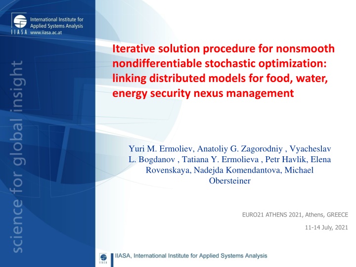
Iterative solution procedure for nonsmooth nondifferentiable stochastic optimization: linking distributed models for food, water, energy security nexus management Yuri M. Ermoliev, Anatoliy G. Zagorodniy , Vyacheslav L. Bogdanov , Tatiana Y. Ermolieva , Petr Havlik, Elena Rovenskaya, Nadejda Komendantova, Michael Obersteiner EURO21 ATHENS 2021, Athens, GREECE 11-14 July, 2021

Advanced Analysis of Interdependencies, Systemic Threats, Multi-Dimensional Systemic risks, and Systemic Security Growing demand vs environmental standards (SDGs); electricity infrastructure innovations and investments; systemic security; increasing returns vs sunk costs; climate change and uncertainty; strategic- and operational planning; long- vs short-term decisions; competition for resources, etc Energy Security Food Security Energy security and water security; supply standards; Energy & water prices; Diversification of energy supply; Ex-ante and ex-post risk management; electricity supply security; global and local threats to electricity supply systems; endogenous risks; cyberattacks; protection of critical infrastructure Incomes; economic and population growth; demand changes; life and nutrition standards; prices; Impacts of energy prices on food prices; Dependencies between agricultural and energy markets through bio-fuels; Agricultural subsidies; renewables subsidies, etc. Nested multi-model welfare analysis and systemic security management Socio - Economic Security Water Security Control of water resources; reliability vs. disasters; Monitoring of infrastructure reliability; monitoring of water resources vulnerability and accessibility; Monitoring & control of water contamination; 2, date

Modeling Challenges Many detailed sectoral models are developed independently by different modeling teams (ministries, authorities, modelers, etc.) The teams are not able to exchange the information about the models (asymmetric information, ASI); Joint resource constraints and supply-demand relations are not accounted for How to link the detailed models under joint constraints and ASI? Traditional integrated modeling (IM) is based on developing and aggregating all relevant (sub)models (sectoral, regional) and corresponding data sets into a single integrated linear programming (LP) model The lack of common information about (LP) submodels makes LP methods inapplicable for integrated LP models Our approach is based on the linkage of separate sectoral/regional LP models under ASI 3, date

Linkage of distributed sectoral/regional models Model of sector/region A Model of sector/region E Minimizing costs , min x c x , min x c x Constraints on volume of production Constraints on available resources (land, water, etc.) A A E E A A R x R x A A x A E E x E M y M y A A A E E E y 0 x D y 0 x D A E d d A A A E E E Constraints are inter- linked! Joint resource constraint + D y D y d A A E E

Nave approach: direct iterative exchange between models Sequential exchange of outputs-inputs between the models Leads to inconsistent solution dependent on initial condition (starting model) The procedure does not converge + ) 1 + ( 1 ), ( x k y k A A , min x c x , min x c x E E A A A A ( ), ( ) x k y k R x R x E E E E x E A A x A M y M y E E E A A A (k ) yE + + ( ) 1 D y D y k d 0 x 0 x A A E E E A (k ) yA + ( ) D y k D y d A A E E + D y D y d A A E E

Hard linking approach: minimization of the overall welfare function Hard linkage within the same programming code Often requires reprogramming and harmonization of inputs Many details of individual models can be lost + , , min c x c x A A E E Ax , x E A x R x R x A A E E x E M y M y A A A E E E 0 x 0 x A E + D y D y d A A E E Implementation may be challenging computing time, needs to re-code etc.

Linking models via a central hub under uncertainty and asymmetric information We reformulate the integrated LP model under ASI as a basic equivalent non- smooth optimization model. For the linkage, the sectorial/regional models don t need recoding or reprogramming. They also don t require additional data harmonization tasks. Instead, they solve their LP submodels independently and in parallel by a specific iterative subgradient algorithm. The submodels continue to be the same separate LP models. A social planner (central hub) only needs to adjust the joint resource constraints to simple subgradient changes calculated by the algorithm. The application of this approach is considered for a case study in Ukraine and China that focuses on the nexus of the agriculture and the energy sectors that are competing for limited water and land resources. 7, date

Linking models via a central hub under uncertainty and asymmetric information We reformulate the integrated LP model under ASI as a basic equivalent non-smooth optimization model. For the linkage, the sectorial/regional models don t need recoding or reprogramming. Instead, they solve their LP submodels independently and in parallel by a specific iterative subgradient algorithm. = + Linkage variable y: , defines constraint on joint resources ) 0 ( ( 0 ( ), 0 ( )) : ) 0 ( ) 0 ( y y y D y D y d A E A A E E + , , ( ) min , u E u y k + , , ( ) min , u A u y k E E E E A A A A E A + R u M c + R u M c E E E E E A A A A A , 0 0 u , 0 0 u E E A A (k ) (k ) A E ) 1 + = + ( ( ( ) ( ) ( )) y k y k k k A Y A A ) 1 + y = y + ( ( ( y ) ( ) ( d )) y y k y k k k E E E E = + {( , : ) E , , 0 0 } Y D D y y A A A E E A E

Iterative procedure Consider ? models of sectors and regions utilizing some common resources. The problem of their linkage can be formulated as follows. Let ?(?) be a vector of decision variables in sector/region ? and assume that each sector/region aims to maximize its net profits ?(?),?(?) ???, (1) subject to constraints ?(?) 0, (2) ?(?)?(?) ?(?), (3) Individual resource constraint ?(?)?(?) ?(?), (4) Joint resource constraint (?) (?), ? = 1,2,...,?. where ?(?),?(?)= ?? ?? ? Here, net unit profits ?(?), vectors ?(?)and matrices ?(?) and ?(?) define the marginal contribution of solutions into the total demand, resource use, and environmental impact. Thus, we distinguish between the constraints (3) that are specific to sector/region k and the constraints (4) that are part of a common inter-sectorial/inter-regional constraint with sectorial/regional (k ) y quotas of resources . 9, date

Iterative procedure Linking the submodels is carried out by linking vectors ?(?). There is a nonempty set of linking vectors ?(?) characterizing the feasible conditions of linkage described by linear constraints . (5) ? ?=1 ?(?)?(?) ? Here matrix ?(?) defines the marginal sectorial/regional resources use with a vector of resources ?, ? 0. The problem of models linkage under full information can be formulated as a total net profit maximization max (6) ? ?=1 ?(?),?(?) s.t. to constraints (2)-(5), ? = 1,2,...,?. By asymmetric information (ASI) of sectors/regions we mean that a sector/region ? does not know ?(?), ?(?), ?(?), ?(?), ?(?) of other sectors/regions, ? ?. Therefore, the integrated LP model (2)-(6) under ASI cannot be solved by LP method due to the lack of common information about submodels. 10, date

Nonsmooth model Let us formulate a basic nonsmooth optimization model that is equivalent to the integrated LP model under ASI. This basic model can be solved by a specific iterative subgradient linkage algorithm. For a given vector ? = (?(1),...,?(?)) let us denote by ?(?) the optimal value of function (6) under constraints (2)-(4). Therefore, , ? ?=1 ?(?)(?) ?(?) = where ?(?)(?) = (?(?),?(?)(?)) are concave nonsmooth functions. In this function ?(?)(?) are optimal solutions of (1)-(4). The required linkage algorithm is defined as a subgradient procedure maximizing function ?(?) s.t. the joint constraints (5). These constraints define the feasible set of the algorithm, which can be denoted also as ?. Therefore, an optimal solutions maximizing ?(?), ? ?, defines also an optimal linkage or a solution of the integrated LP model under ASI. In the following we assume the existence of solutions ?(?)(?), ? ?, for all ?. 11, date

Iterative linking. Let us consider a sequence of approximate solution ??= (??(1),...,??(?)) for iteration ? = 1,2, of the algorithm. For given quotas ?? independently and in parallel, sectors/regions solve models (1)-(4), ? = 1,2, ,?, and obtain primal solutions ??(?)= ??(?)(??) together with the corresponding solutions (??(?),??(?)) of the dual problems ?(?),?(?)+ ?(?),?(?) min, (7) ?(?)?(?)+?(?)?(?) ?(?), (8) ?(?) 0,?(?) 0, ? = 1,2, ,?. (9) The next approximation ??+1= ??+1(1), ,??+1(?) is derived by a social planner (hub) as ??+1= ??(??+????), ? = 1,2,..., (10) where ?? is an iteration-dependent step-size multiplier and ?? is the orthogonal projection operator onto set ?. Vector ?? is a generalized gradient or a subgradient of function ?(?) at ? = ??. The step-size ?=1 ?? is chosen from rather general and natural requirements: ?? 0, ?? 0, ??= 1/?), because subgradients (generalized gradients) are not, in general, the increasing directions of functions. = , (e.g. ?? The proposed linkage algorithm for problems under ASI (10) requires additional condition ?=1 < to enable the convergence of not only function ?(??) but also of the solutions ?? 2 ?? This allows us to propose a simple stopping criterion (see Step 4, Algorithm) enabling parallel 12, date optimization of interdependent sectors by (10).

Convergence theorem =1 k = = ( ) 0 : ( ) , 0 , ( ) k k k k Let = Then * * A * E ( ) ( ( ), ( )) ( , ) y k y k y k y y y A E + y = * * Ay * , , min , x E c x c x ( , : ) E y where A A E E , , x y y A A E & R x R x A A x A E E x E y & M y M A A A E E E 0 & 0 x x A E 0 & 0 y y A E Yuri Ermoliev (1988), Yuri Ermoliev et al. ( 2017, 2019) for Deterministic and stochastic cases

Iterative procedure Algorithm. There is a network of distributed computers connecting submodels, say sectors, with a central hub computer. The linkage algorithm can be summarized as follows: Step 0: Initialization. Sector ?, ? = 1,...,?, chooses initial vectors ?0(?) of resource quotas and submits it to the central computer (hub). The computer projects ?0= (?0(1),...,?0(?)) onto the set ? defining a first feasible approximation?1= (?1(1),...,?1(?)); set ? = 1 Step 1: Generic step. Suppose by the beginning of iteration ? the algorithm arrived at vector ??= (??(1),...,??(?)). Then on iteration ? the algorithm proceeds as follows. Step 2: All sectors ? receive ??(?) and solve models (1)-(4) independently. Shadow prices ??(?) of common resources (constraints (4)) are submitted to the central computer (hub). Step 3: The central computer calculates ??+???? with a step-size ??= ??/?, where ?? is a scaling parameter, ? ?? ? for some constants ?, ?. It regulates ?? so that the product ???? corresponds to the scale of ??. Vector ??+???? is projected onto the set ? and defines ??+1. Sectorial/regional computers receive corresponding components of ??+1. Step 4: All sectors independently check stopping criteria. Sector ? calculates non-negative difference ??(?)= (?(?),??(?)(??))+(??(?),??(?)(??)) ??(?(?),??(?)(??)) and submits values ??(?) to the central computer of the hub. If ?? continues with an itteration increment of 1 and returns to step 1. (?) ? 0, where ? is an admissible accuracy, then the algorithm stops. Otherwise, it ? 14, date

Convergence. Consider the sectorial/regional model k defined by equations (1)-(4) for a given feasible ? satisfying the constraints (5). ( ) xk ( ) Proposition (Stoping criterion, subgradients): Assume there exist solutions y of all Ksectorial/regional models. Then: a). Functions ? ? ? = (?(?),?(?)(?)), ?(?) = non-differentiable functions for all ?. ? ?=1 are concave continuously ?(?)(?(?)) b). The dual problem (7)-(9) has a solution (?(?)(?),?(?)(?)) for all ?, and these solutions satisfy the stopping criterion of the linkage algorithm: ?(?)(?) = (?(?),? (?)) = (?(?),? (?))+ (?,? (?)). From this proposition follows the following fact (Ermoliev, 1976; Rockafeller, 1981), which is fundamental for solving the linkage problem through maximizing non-differentiable function ?(?) by algorithm (10). c). For any feasible solution ? and ?, ?(?)(?) ?(?)(?) (?(?)(?),? ?), that is, ?(?)(?) is a sub-gradient of the concave non-differentiable function ?(?)(?). Vector ?(?) = ? ?=1 (?(1)(?),...,?(?)(?)) is a sub-gradient of function?(?) = , ??(?) = ?(?), that ?(?)(?) is, ?(?) ?(?) (?(?),? ?). 15, date

On linking under food-energy-water-land nexus in China Application of the proposed iterative linkage algorithm in the case study linking location- specific energy (coal) and agricultural sectorial models. Both separate models are used for optimal energy and agricultural production planning in the water-scarce Shanxi region in China (Gao et al.,2018). In the following, we present a description of the models structure, main parameters and decision variables. In short, the integrated model can be summarized as follows. The model consists of two submodels, the energy and the agricultural production planning models. Both models are spatially detailed, which allows also to link the models across locations and thus control local drivers having significant implications on the overall results of models integration. The model accounts for various coal mining, processing and conversion technologies, as well as for various types of crops in a number of locations within the region. Coal and agricultural production are restricted by the availability of water and land. Coal-based industries mining, washing, chemical production, and power generation are all extremely water-intensive. About 53% of China s coal reserves are located in water scarce regions, while 30% are in water stressed regions and Shanxi is one of them. Water supply to agriculture can significantly improve rural developments and maintain food security. 16, date

Linkage of distributed energy-agriculture-water models Coal related industry Cooling technology Power Waste water treatment dry quenching coke Power reuse Waste water treatment Coal Mining Water resource Quantity Water resource Quality Coal quantity Dry/reuse of water Drainage water Agriculture Crop stucture crop quantity Air Pollution 17, date

Energy, water, and agricultural nexus In the integrated model, a social planner (hub) chooses decisions ?????? on how much coal of type ?,? = 1, ,? to exctract in location ?,? = 1, ,?, transport to location ?, ? = 1, ,?, and convert by technology ?. In addition, decisions ???? are made on how much agricultural commodities k, ? = 1, ,? to produce in location j and export to location ? so that the total costs from the coal (energy sector) and agricultural production, transportation, and conversion is minimized. Individual sectorial models. The sectorial goal functions are as follows ??+???? ??+???? ?? ????? ??? (12) ??? ?,?,?,?,? and ??+??? ?? ???? ??? (13) ??? ?,?,?,?,? ?? stands for for the coal-based energy production and agricultural sectors, respectively. Here ??? ?? - transportation cost of the production cost for a unit (i.e., ton) of coal (type) ? in location ?, ???? ?? is the conversion costs for a unit of coal ? by a unit of coal ? from location ? to location ?, ???? ?? denotes costs associated with production of a unit agricultural technology ? in location ?, ??? ?? is the transportation cost for a unit of the agricultural commodity ? in location ?, and ???? commodity ? from location ? to location ?. 18, date

Energy and food security interdependencies. Demand for useful or final energy converted from coal, for example, electricity, which accounts for more than half of total coal conversion in China, heat, coke, gas, and oil. Thus, there is a constraint on the energy produced from coal as follows: ? ?, (14) where ???? end-product of type ?, and ?? ???? ????? ?? ??? ? denotes the conversion efficiency of coal type ? in location ? by technology ?, the ? stands for the end product demand ?. There is a constraint that defines the minimum required production level of agricultural commodity k in location ? as follows: ?, (15) ???? ? where ??? terms of the minimum amount of daily calories required per capita suggested by the World ??? ? is the demand for agricultural commodity ? in location m. ??? ? can be measured in Health Organization (WHO) accounting for size, age, sex, physical activity, climate, and other factors. 19, date

Natural resource constraints. Sectorial land constraints in Shanxi region ? (16) (1 ??? ??????+? ????? ????? ?? ?,?,? ?,?,? and ? (17) ??????? ?? ?,? ? and ?? ? in incorporate exogenous assumptions on land allocated for coal and crop production ?? locations ?, for the coal and agricultural sectors respectively; Here ??? is the area of land that subsides as a result of mining a unit of coal of type ? in location ?, ??? represents the fraction of the farmland overlapped with the coal filed in the location ?, and ??? stands for the land reclamation rate (or efficiency rate) for coal ? in location ?, and ? is a coefficient related to separating coal from other materials. Also, ??? stands for the area of farmland required for the production of a unit of crop ? in location ?. There are constraints on total available land ?? in each location ? ??. (18) + (1 ??? ??????+? ??????? ????? ????? ?,? ?,?,? ?,?,? Water quotas allocated to the sectors limit the choice of coal and crop production technologies ?+??? ?]????? ?, (19) [??? ?? ?,?,? and ????? ?, (20) ??? ?? ?,? ? and ?? ? define water provided to the coal (energy) and agricultural sectors in location where ?? ?, ??? amount of water required to convert a unit of coal ? in location ?, ??? required to irrigate a unit of crop k in location j, and ?? defines water availability in location ?. Constraint on the water ?? water ?? ? defines the amount of water required to produce a unit of coal ? in location ?, ??? ? is the ? is the amount of water ? required for coal production, processing, and conversion and on the ? for crop irrigation purposes in each location?: 20, date ?+?? ? ??. (21) ??

Model linkage. In order to demonstrate the applicability of algorithm (10) for linking distributed models under ASI let us ignore in the following the existence of full common information about LP submodels (12), (14), (16), (19) and (13), (15), (17), (20). To link the energy ((12), (14), (16), (19)) and the agricultural ((13), (15), (17), (20)) sectorial models in such a way that joint constraints (18) and (21) are fulfilled, we implement the procedure (10). The linkage of the models is accomplished as follows: At the initial step s=0, individual sectorial models are solved using reasonable assumptions on ?(0), ?? ?(0) and ?? ?(0), ?? ?(0) between the sectors. resource distribution ?? The resource distribution ?? at step ? is adjusted according to (10) using shadow prices (dual variables) of the constraints ?(? 1) (22) (1 ???)??????+? ????? ????? ?? ?,?,? ?,?,? ?(? 1), (23) ??????? ?? ?,? ?????? ?????? ?(? 1), (24) + ??? ??? ?? ?,?,? ?,?,? ????? ?(? 1), (25) ??? ?? ?,? and constraints (18), (21). It is important that the proposed approach allows to link models under asymmetric information on remote computers. 21, date

Figure 1 presents the values of the total cost function in each iteration of the algorithm for three different scenarios of initial water and land allocation quotas between the energy and the agricultural production sectors. The iterative process converges rather quickly. In 10 iterations the optimal value of the integrated (linked) model is almost equal to the value of the hard-linked model, i.e. the optimal water and land quotas are found. Model Net profit, Total, bln. CNY Net profit, Agriculture, bln. CNY Net profit, Energy, bln. CNY Two separate sectorial optimizations (no joint constraints) 254.2 17.7 236.5 Integrated hard-linked 176.0 13.9 162.1 Integrated linked via a central hub 177.3 13.9 163.4 Table 1: Optimal net profits (values of goal functions) for three cases: 1. separately optimized models; 2. the hard-linked models; 3. integrated (linked via a central hub) model. 22, date

Figure 1: Convergence (in terms of net profts (the goal function value) of the iterative linking procedure to the solution of the hard-linked problem. The values of net profits are on the vertical axis and the iteration number is on the horizontal axis. The three curves (Sc1, Sc2, Sc3) correspond to three different initial water quata allocation scenarios (at s = 0). Figure 1 demonstrates the nonmonotonic convergence of values ?(??) because the total net profit is not a continuously differentiable function. An essential factor affecting the convergence speed of non-monotonically changing objective function is the choice of the step-size ??. A general rule is that the scale of the product ???? must correspond to the scale of the solutions??. 23, date

Concluding remarks This paper presented two novel results. First, it is the algorithm that allows the social planner (hub), who pursues the total net cost minimization, to distribute limiting resources between sectors/regions without knowing their models. The algorithm requires only the shadow prices for the individual resource bounds. More specifically, this method links different separate LP models into a single integrated model without re-coding, re-programming and data harmonization. Second, the paper demonstrates the applicability of the algorithm with an example of linking two location-specific sectorial models, the energy (coal) and agricultural models, under a common water resource constraint in a coal-rich and water-scare Shanxi region, in China. The proposed computational algorithm is based on subgradient methods invented for the optimization of non-smooth systems, which may be subject to shocks and discontinuities. Therefore, these methods will be naturally the algorithm is developed further for linking stochastic sectorial models with known marginal distributions of sectorial uncertainties, into cross-sectorial integrated models with joint distributions of collective systemic risks induced by sectorial uncertainties and decisions maximizing a stochastic version of the function (6). It is worth noting that the algorithm can also carry out the linkage of dynamic systems. Fundamentally important possible extension of the presented method is the case of stochastic sectorial/regional models with interdepedent uncertainties, which can be shaped by linking decisions of various agents. The mitigation of floods by new land use decisions, for example, affect flood scenarios. As a rule, this makes it impossible to separate scenario generations and optimization processes calling for linking both simulation and optimization procedures in a similar manner to algorithm (10), thus combining simulations of scenarios, new optimization steps, new simulation of scenarios, and so on. In this case we can think of new type machine 24, date learning processes. While in this paper, we meant linking regional and/or sectorial models when referring to model linkage, more generally, linking models may refer to different local-global scales. Therefore, the linkage problem can also be formulated much more generally in terms of sub-models and integrated models and the approach presented in this paper can still be applicable. Remark 2 illustrates this in more detail.