Jacobi and Gauss-Seidel Iterative Techniques for Linear Systems
In Section 11.2, the Jacobi and Gauss-Seidel iterative methods are described for solving linear systems. The approach involves altering the coefficients on the left-hand side of the equations to simplify the iterative process. Through examples and explanations, the methods for solving linear systems using these techniques are elucidated step by step.

Download Presentation

Please find below an Image/Link to download the presentation.
The content on the website is provided AS IS for your information and personal use only. It may not be sold, licensed, or shared on other websites without obtaining consent from the author.If you encounter any issues during the download, it is possible that the publisher has removed the file from their server.
You are allowed to download the files provided on this website for personal or commercial use, subject to the condition that they are used lawfully. All files are the property of their respective owners.
The content on the website is provided AS IS for your information and personal use only. It may not be sold, licensed, or shared on other websites without obtaining consent from the author.
E N D
Presentation Transcript
Sec:11.2 The Jacobi and Gauss- Siedel Iterative Techniques
Sec:11.2 The Jacobi and Gauss-Siedel Iterative Techniques In this section we describe the Jacobi and the Gauss-Seidel iterative methods We want to solve the following linear system 6 x 10 -1 2 0 -1 11 -1 3 2 -1 10 -1 0 3 -1 8 ? 1 25 x 2 = 15 ? 11 x 3 ?? = ? x ? 4 Example solve the linear system + = 10 2 + 6 x x x 1 2 3 + = 11 3 25 x x x x 1 2 3 4 + = 2 10 11 x x x x 1 2 3 4 = 3 8 15 x x x 2 3 4
Sec:11.2 The Jacobi and Gauss-Siedel Iterative Techniques We want to solve the following linear system Example Keep the diagonal on the left hand side solve the linear system = + 10 = 2 6 x x x + = 10 2 + 6 x x x 1 2 3 1 2 3 + + + = 11 = + 3 25 x x x x 11 3 25 x x x x 2 1 3 4 1 2 3 4 + = + 2 10 11 x x x x 10 2 + 11 x x x x 1 2 3 4 3 1 2 4 = 3 8 15 x x x = + 8 3 15 x x x 2 3 4 4 2 3 Jacobi Iterative Method Change the coeff of LHS to be one by division From the initial approx. ?(?)= (?,?,?,?)?we ?(?) = / ) 6 + = = / ) 6 + 25 ) 1 ( 1 x ) 0 ( 2 ) 0 ( 3 ( ( 2 + 3 + 10 / ) ( 2 10 x x x x x x x 1 2 3 + + x 11 x x 2 1 3 4 = + + ) 1 ( 2 x ) 0 ( 1 x ) 0 ( 3 ) 0 ( 4 ( + x 3 25 / ) 11 x x = ( 2 + 11 + / ) 10 x x x 3 1 2 x 4 = + ) 1 ( 3 x ) 0 ( 1 x ) 0 ( 2 ) 0 ( 4 ( 2 + x 11 / ) 10 x ( = ) 8 3 15 ) /( x x 4 2 3 ( = + ) 8 ) 1 ( 4 x ) 0 ( 2 ) 0 ( 3 3 15 ) /( x
Sec:11.2 The Jacobi and Gauss-Siedel Iterative Techniques From the initial approx. ?(?)= (?,?,?,?)?we ?(?) = / ) 6 + ) 1 ( 1 x ) 0 ( 2 ) 0 ( 3 ( 2 10 x x . 0 600 0 6 / 10 . 2 272 0 25 / 11 = + + ) 1 ( 2 x ) 0 ( 1 x ) 0 ( 3 ) 0 ( 4 ( + x 3 25 / ) 11 x x = = = (x ) 0 ) 1 (x . 1 100 0 11 / 10 = + ) 1 ( 3 x ) 0 ( 1 x ) 0 ( 2 ) 0 ( 4 ( 2 + x 11 / ) 10 x . 1 875 0 15 8 / ( = + ) 8 ) 1 ( 4 x ) 0 ( 2 ) 0 ( 3 3 15 ) /( x Jacobi Iterative Method From the k-th approx. ?(?)= (?,?,?,?)?we ?(?+?) . 0 600 ) 1 + = / ) 6 + . 1 047 ( ( 2 ) ( 3 ) k k k ( 2 10 x x x 1 . 2 272 . 1 715 = ) 1 (x = (x 2 ) ) 1 + = + + ( 2 ( ) ( 3 ) ( 4 ) k k k k ( + x 3 25 / ) 11 x x x x . 1 100 . 0 805 1 ) 1 + = + . 1 875 ( 3 ( ) ( 2 ) ( 4 ) k k k k ( 2 + x 11 / ) 10 x x x . 0 885 1 ) 1 + ( = + ) 8 ( 4 ( 2 ) ( 3 ) k k k 3 15 ) /( x x
Sec:11.2 The Jacobi and Gauss-Siedel Iterative Techniques Jacobi Iterative Method 0 ) 1 + = / ) 6 + ( ( 2 ) ( 3 ) k k k ( 2 10 x x x 1 0 = (x ) 0 ) 1 + = + + ( 2 ( ) ( 3 ) ( 4 ) k k k k ( + x 3 25 / ) 11 0 x x x x 1 0 ) 1 + = + ( 3 ( ) ( 2 ) ( 4 ) k k k k ( 2 + x 11 / ) 10 x x x 1 ) 1 + ( = + ) 8 ( 4 ( 2 ) ( 3 ) k k k 3 15 ) /( x x ? = ? 0.6000 1.0473 0.9326 1.0152 0.9890 2.2727 1.7159 2.0533 1.9537 2.0114 -1.1000 -0.8052 -1.0493 -0.9681 -1.0103 1.8750 0.8852 1.1309 0.9738 1.0214 ? = ? ? = ? ? = ? ? = ? (?) ?? (?) ?? (?) ?? (?) ?? ? = 6 1.0032 0.9981 1.0006 0.9997 1.0001 1.9922 2.0023 1.9987 2.0004 1.9998 -0.9945 -1.0020 -0.9990 -1.0004 -0.9998 0.9944 1.0036 0.9989 1.0006 0.9998 ? = 7 ? = 8 ? = 9 ? = 10 1 (?) ?? 2 (?) = *x ?? 1 1 (?) ?? (?) ??
Sec:11.2 The Jacobi and Gauss-Siedel Iterative Techniques Gauss Seidel Method From the k-th approx. ?(?)= (?,?,?,?)?we ?(?+?) ) 1 + = / ) 6 + ( ( 2 ) ( 3 ) k k k ( 2 10 x x x 1 Note that in the Jacobi iteration one does not use the most recently available information. ) 1 + = + + ( 2 ( ) ( 3 ) ( 4 ) k k k k ( + x 3 25 / ) 11 x x x x 1 ) 1 + = + ( 3 ( ) ( 2 ) ( 4 ) k k k k ( 2 + x 11 / ) 10 x x x 1 ) 1 + ( = + ) 8 ( 4 ( 2 ) ( 3 ) k k k 3 15 ) /( x x From the k-th approx. ?(?)= (?,?,?,?)?we ?(?+?) ) 1 + = / ) 6 + ( ( 2 ) ( 3 ) k k k ( 2 10 x x x 1 ) 1 + ) 1 + = + + ( 2 ( ( 3 ) ( 4 x ) k k k k ( + x 3 + 25 / ) 11 x x x x 1 ) 1 + ) 1 + ) 1 + = ( 3 ( ( 2 ( 4 ) k k k k ( 2 + x 11 / ) 10 x x 1 ) 1 + ) 1 + ) 1 + ( = + ) 8 ( 4 ( 2 ( 3 k k k 3 15 ) /( x x ? = ? ? = ? ? = ? ? = ? ? = ? (?) ?? 0.6000 1.0302 1.0066 1.0009 1.0001 2.3273 2.0369 2.0036 2.0003 2.0000 -0.9873 -1.0145 -1.0025 -1.0003 -1.0000 0.8789 0.9843 0.9984 0.9998 1.0000 Note that Jacobi s method in this example required twice as many iterations for the same accuracy. (?) ?? (?) ?? (?) ??
Sec:11.2 The Jacobi and Gauss-Siedel Iterative Techniques a a x b 11 1 1 1 n Jacobi iteration for general n: = a a x b = for i : 1 n 1 n nn n n 1 i n = = + = ( ) 1 ( ) ( ) k k k x b a x a 1 x a i i ij j ij j ii + 1 j j i end Gauss-Seidel iteration for general n: = for i : 1 n 1 i n = = + + = ( ) 1 ( ) 1 ( ) k k k x b a x a 1 x a i i ij j ij j ii + 1 j j i end
Sec:11.2 The Jacobi and Gauss-Siedel Iterative Techniques Example Splittings and Convergence Splitting DEF: A 0 3 10 0 0 0 0 0 0 0 0 8 1 0 0 10 1 2 0 1 11 1 3 2 0 0 1 2 1 0 1 11 0 0 3 1 0 1 10 1 = = 1 8 10 0 2 0 1 M N 3 Ax = b A large family of iteration ( ) = + Nx + M Mx N Nx = M = = x b b ) 1 + = + ( ( ) k k x Tx b = 1 T M N where + 1 1 x M b b x Tx
Sec:11.2 The Jacobi and Gauss-Siedel Iterative Techniques Example: 10 -1 2 0 -1 11 -1 3 2 -1 10 -1 0 3 -1 8 A large family of iteration 6 x b ) 1 + = + ( ( ) k k 1 x Tx 25 x 2 = 15 11 x 3 = 1 T M N where x 4 U L D A 10 1 -2 0 1 -3 10 -1 2 0 -1 11 -1 3 2 -1 10 -1 0 3 -1 8 -2 1 0 -3 1 ) U = 11 1 10 1 8 = + ( A D L GS: Jacobi: = = = = = + , , ( ) M = D L N U M D N L U 1 + 1 ( ) TGS D L U ( ) TJ D L U
Sec:11.2 The Jacobi and Gauss-Siedel Iterative Techniques = + + ( ) Dx L U x b We want to solve the following linear system Example Keep the diagonal on the left hand side solve the linear system = + 10 = 2 6 x x x + = 10 2 + 6 x x x 1 2 3 1 2 3 + + + = 11 = + 3 25 x x x x 11 3 25 x x x x 2 1 3 4 1 2 3 4 + = + 2 10 11 x x x x 10 2 + 11 x x x x 1 2 3 4 3 1 2 4 = 3 8 15 x x x = + 8 3 15 x x x 2 3 4 4 2 3 + = ( ( )) D L U x b Change the coeff of LHS to be one by division Jacobi Iterative Method = = / ) 6 + 25 ( ( 2 + 3 + 10 / ) x x x x x 1 2 3 + + x 11 x x 2 1 3 4 = ( 2 + 11 + / ) 10 x x x = + + 1 1 3 1 2 x 4 ( ) x D L U x D b ( = ) 8 3 15 ) /( x x 4 2 3
Sec:11.2 The Jacobi and Gauss-Siedel Iterative Techniques GS: Jacobi: = = = = = + , , ( ) M = D L N U M D N L U 1 + 1 ( ) TGS D L U ( ) TJ D L U A=[10 -1 2 0;-1 11 -1 3;2 -1 10 -1;0 3 -1 8]; b = [6; 25; -11; 15]; U=-triu(A,1); L=-tril(A,-1); D=diag(diag(A)); A=[10 -1 2 0;-1 11 -1 3;2 -1 10 -1;0 3 -1 8]; b = [6; 25; -11; 15]; U=-triu(A,1); L=-tril(A,-1); D=diag(diag(A)); TJ= D\(L+U); bJ = D\b; Tgs=(D-L)\U; bg = (D-L)\b; x=[0; 0; 0; 0]; for i=1:10 x = TJ*x + bJ; end x x=[0; 0; 0; 0]; for i=1:5 x = Tgs*x + bg; end x
Sec:11.2 The Jacobi and Gauss-Siedel Iterative Techniques GS: Jacobi: = = = = = + , , ( ) M = D L N U M D N L U 1 + 1 ( ) TGS D L U ( ) TJ D L U A large family of iteration THM: b ) 1 + = + ( ( ) k k x Tx Convg All eigenvalues of T in absolute value are less than one. n , , 1 = 1 T M N where 1 DEF: Example Let A be nxn matrix with eigenvalues , i = , 2 i 2 1 2 i n , 1 = 1 0 0 A i , 1 , 1 = ) = A 2 spectral radius of A is defined to be 0 1 0 ( 2 = ( ) max , , , A 1 2 n
Sec:11.2 The Jacobi and Gauss-Siedel Iterative Techniques A large family of iteration THM: b ) 1 + = + ( ( ) k k x Tx Convg ( ) 1 T = 1 T M N where
Sec:11.2 The Jacobi and Gauss-Siedel Iterative Techniques U L D A 10 1 -2 0 1 -3 10 -1 2 0 -1 11 -1 3 2 -1 10 -1 0 3 -1 8 -2 1 0 -3 1 = 11 1 10 1 8 Jacobi: ( M GS: = 0.4264 = + = ) = , ( ) , M = D N L U M D L N U gsN = JN 1 1 ( 0.0898 M ) gs J A=[10 -1 2 0;-1 11 -1 3;2 -1 10 -1;0 3 -1 8] U=-triu(A,1) L=-tril(A,-1) D=diag(diag(A)) THM: ( ) 1 T TJ= D\(L+U) Tgs=(D-L)\U Convg max(abs(eig(TJ))) 0.426436610842342 max(abs(eig(Tgs))) 0.089823058388043
Sec:11.2 The Jacobi and Gauss-Siedel Iterative Techniques Convergence Criterion for the Gauss-Seidel Method A large family of iteration THM: b ) 1 + = + ( ( ) k k x Tx Convg ( ) 1 T = 1 T M N where We can now give easily verified sufficiency conditions for convergence of the Gauss- Seidel methods. Definition A is strictly diagonally dominant That is, the diagonal coefficient in each of the equations must be larger than the sum of the absolute values of the other coefficients in the equation ? ???> ???, ??? ??? ? ?=1 ? ?
Sec:11.2 The Jacobi and Gauss-Siedel Iterative Techniques Convergence Criterion for the Gauss-Seidel Method Definition A is strictly diagonally dominant That is, the diagonal coefficient in each of the equations must be larger than the sum of the absolute values of the other coefficients in the equation ? ???> ???, ??? ??? ? ?=1 ? ? Example2 Example1 A A 10 -1 2 0 -1 4 2 -1 4 -1 0 3 -1 2 10 -1 2 0 -1 11 -1 3 2 -1 10 -1 0 3 -1 8 -1 3 THM: GS Convg A is strictly diagonally dominant
Sec:11.2 The Jacobi and Gauss-Siedel Iterative Techniques Example1 Definition The L2 norms for the vector ? are defined by 3 2 ? = ?1 ?? 1 2+ ?2 2+ + ?? 2 ? = ?1 ? = ? = 14 norm of the vector x = (x1, x2, x3)t gives the length of the straight line joining the points (0, 0, 0) and (x1, x2, x3). the distance between two vectors is defined as the norm of the difference of the vectors
Sec:11.2 The Jacobi and Gauss-Siedel Iterative Techniques A=[10 -1 2 0;-1 11 -1 3;2 -1 10 -1;0 3 -1 8]; b = [6; 25; -11; 15]; U=-triu(A,1); L=-tril(A,-1); D=diag(diag(A)); function [x,iter] = gauss_seidel(A,b,x0,tol) U=-triu(A,1); L=-tril(A,-1); D=diag(diag(A)); Tgs=(D-L)\U; bg = (D-L)\b; Tgs=(D-L)\U; bg = (D-L)\b; imax=200; iter=imax; xold = x0; for i=1:imax x = Tgs*xold + bg; dif = norm(x-xold); resd = norm(b-A*x); xold = x; if dif < tol & resd < tol; iter =i;break; end; end; end x=[0; 0; 0; 0]; for i=1:5 x = Tgs*x + bg; end x Stopping Criteria: ?? = ? residual ? ??(?) < ??? ?(?+1) ?(?) < ??? clear; clc A=[10 -1 2 0;-1 11 -1 3;2 -1 10 -1;0 3 -1 8]; b = [6; 25; -11; 15]; x0=[0; 0; 0; 0]; tol=1e-4; [x,iter] = gauss_seidel(A,b,x0,tol) Example: 10 -1 2 0 -1 11 -1 3 2 -1 10 -1 0 3 -1 8 6 x 1 25 x 2 = 15 11 x 3 x 4