Kinematics and Kinetics in Engineering Dynamics

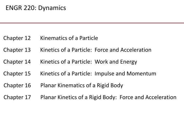
ENGR 220: Dynamics Chapter 12 Kinematics of a Particle Chapter 13 Kinetics of a Particle: Force and Acceleration Chapter 14 Kinetics of a Particle: Work and Energy Chapter 15 Kinetics of a Particle: Impulse and Momentum Chapter 16 Planar Kinematics of a Rigid Body Chapter 17 Planar Kinetics of a Rigid Body: Force and Acceleration

12.1 Introduction MECHANICS STATICS DYNAMICS (objects in equilibrium) (objects in motion) KINETICS KINEMATICS (geometric aspects of motion) (analysis of forces causing motion) Chapter 12 Kinematics of a Particle

12.2 Rectilinear Kinematics: Continuous Motion Velocity: Change in position. ? =?? instantaneous velocity is the time derivative of position EQ 12 1 ?? Acceleration: Change in velocity. ? =?? instantaneous acceleration is the time derivative of velocity ?? EQ 12 2 Relationship between position, velocity, and acceleration: ds v dv a = ads vdv = (EQ 12-3 ) With no time dependance

12.2 Rectilinear Kinematics: Continuous Motion a a = Special Case: Constant Acceleration c = v v = = Integrate , assuming when 0 a dv dt t Velocity as a Function of Time: 0 c v t ( ) v v = + = EQ 12- 4 dv a dt a t 0 c c 0 v 0 Position as a Function of Time: v ds dt v = = + s s = = Integrate , assuming when 0 a t t 0 0 c s t ( ) ( ) + s s = + + 1 2 = EQ 1 2-5 ds v a t dt v t a t 2 0 0 0 c c 0 s 0 vdv a ds = v v = s s = Integrate , assuming when Velocity as a Function of Position: 0 0 c v s ( ) ( ) = + = 2 EQ 12-6 vdv a ds v v a s s 2 2 0 0 c c v s 0 0

12.3 Rectilinear Kinematics: Erratic Motion In many cases the position, velocity, and acceleration of a particle cannot be described by a continuous mathematical function along its entire path. The s-t and v-t graphs: ds dt= v slope of = velocity s-t graph

12.3 Rectilinear Kinematics: Erratic Motion In many cases the position, velocity, and acceleration of a particle cannot be described by a continuous mathematical function along its entire path. The v-t and a-t graphs: dv dt= a slope of = acceleration v-t graph

Relationship Between s-t, v-t, and a-t Graphs How about the other way? What if you have a plot of acceleration as a function of time? How to you get to velocity? Or position? You know that: = = v adt s vdt change in velocity area under a-t graph area under = displacement = v-t graph In theory, if I gave you a plot of acceleration vs. time, and some grid paper, you could probably draw me a pretty accurate velocity vs. time plot.

12.3 Rectilinear Kinematics: Erratic Motion In many cases the position, velocity, and acceleration of a particle cannot be described by a continuous mathematical function along its entire path. The a-t and v-t graphs: = v adt change in velocity area under a-t graph =

12.3 Rectilinear Kinematics: Erratic Motion In many cases the position, velocity, and acceleration of a particle cannot be described by a continuous mathematical function along its entire path. The v-t and s-t graphs: = s vdt area under displacement = v-t graph

12.5 Curvilinear Motion: Rectangular Components A particle located at (x,y,z) from origin 0. Position: ( ) = + + r i j k EQ 12- 10 x y z position: = + + r x y z 2 2 2 magnitude: Velocity has direction and magnitude. Velocity is always tangent to the path. Tail emanates from the particle. Velocity: r d dt d dt d dt d dt d dt dx dt dy dt dz dt = = = vector velocity: ( ) x ( ) y ( ) = = + + = + + v i j k i j k i j k , , ( ) z f t r v v v x y z ( ) = = + + v i j k x EQ 12-11 v v v ( ) x y z EQ 12-12 y z = + + v v v y 2 x 2 y 2 z magnitude:

12.5 Curvilinear Motion: Rectangular Components Acceleration has direction and magnitude. Acceleration points towards the inside of the path curve. Acceleration: v d dt vector acceleration: ( ) = = = a a a x y z = = + + a i j k EQ 12-13 a a a x x y z ( ) EQ 12-14 y z = + + a a a a 2 x 2 y 2 z magnitude:

12.6 Motion of a Projectile Free-flight motion of a projectile using rectangular components. Assumptions for Analysis: constant acceleration (no variation with altitude or elevation) no friction/damping from air (no forces act on particle during flight) = + + + v v x x = = a t v t ??= ? = 9.81 m s2= 32.2 ft Constant Acceleration Equations: 0 c + 1 2 x x a t 2 s2 0 2 0 0 a c ( ) 2 v v 2 0 c For projectile flight, use: = = 0 & a a g x y ( ) v = v Horizontal Motion: 0 x x x = x ( ) v + t 0 0 x = = = ( ) v y v v gt 0 y y y Vertical Motion: + 1 2 ( ) v t gt 2 0 0 y ( ) 2 ( g y y ) v 2 y 2 y 0 0

12.7 Curvilinear Motion: Normal and Tangential Components Planar Motion: Coordinate system has origin at a fixed point on the curve, and at the instant considered this origin happens to coincide with the location of the particle. u u (tangential unit vector) (normal unit vector) t Position: n The tangential direction, t is tangent to the path and points in the direction of motion. = v u (EQ 12-15 ) v t Velocity: The normal direction, n is perpendicular to the tangential direction and points to the instantaneous center of curvature 0 . v s = (EQ 12-16)

12.7 Curvilinear Motion: Normal and Tangential Components Acceleration Analysis: Acceleration is time rate of change of velocity: = = a v + u u u 0! v v t t t = = = u u & & d d ds d s t n s v = = = u u u u t n n n Acceleration: = + a u u (EQ 12-18) a a t t n n = v (EQ 12-19) a v t 2 = (EQ 12- 20) a n = + a a a 2 t 2 n magnitude:

12.8 Curvilinear Motion: Cylindrical Components u (radial unit vector) (transverse unit vector) u r Polar Coordinates: = r u r Position: r Velocity: = = v r + u u r r r r = = v r + = u u u u r r r r = = v r + u u (EQ 12-24) v v r r = = r v v r r (EQ 12-25) velocity magnitude: = + r ( ) r ( ) v 2 2

12.8 Curvilinear Motion: Cylindrical Components u (radial unit vector) (transverse unit vector) u ( r r r dt r r r = = + + a v u u r Polar Coordinates: d ) = = a v + u u Acceleration: + + u u u r r r r = = a v r r + + = = u u u u u u ( ) ( 2 ) & r r 2 r r r = + a u u (EQ 12-28) a a r r = = + r a a r r r 2 (EQ 1 2-29) 2 r Acceleration magnitude: = r r + + ( 2 2 ) ( 2 ) a r r 2

12.9 Absolute Dependent Motion Analysis of Two Particles The motion of one particle depends directly on the motion of another particle. Example 1: Example 2: h s + + = 2B s l A + = = 2 0 or 2 v v v v B A B A + = = 2 0 or 2 a a a a B A B A + + = s CD l s l A B T + = = 0 or v v v v A B B A + = = 0 or a a a a A B B A

12.10 Relative-Motion of Two particles Using Translating Axes Translating frame of reference is attached to and moves with particle A. = + r r B A r Position: B A = + v v v Velocity: B A B A = + a a a Acceleration: B A B A