Kohonen Self-Organizing Maps for Categorizing Input Vectors

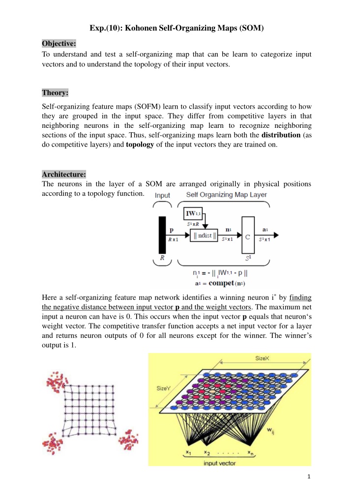
Exp.(10): Kohonen Self-Organizing Maps (SOM) Objective: To understand and test a self-organizing map that can be learn to categorize input vectors and to understand the topology of their input vectors. Theory: Self-organizing feature maps (SOFM) learn to classify input vectors according to how they are grouped in the input space. They differ from competitive layers in that neighboring neurons in the self-organizing map learn to recognize neighboring sections of the input space. Thus, self-organizing maps learn both the distribution (as do competitive layers) and topology of the input vectors they are trained on. Architecture: The neurons in the layer of a SOM are arranged originally in physical positions according to a topology function. Here a self-organizing feature map network identifies a winning neuron i* by finding the negative distance between input vector p and the weight vectors. The maximum net input a neuron can have is 0. This occurs when the input vector p equals that neuron s weight vector. The competitive transfer function accepts a net input vector for a layer and returns neuron outputs of 0 for all neurons except for the winner. The winner s output is 1. 1

Kohonen Learning Rule (learnk): The function learnk is used to perform the Kohonen learning rule for SOM nets. The weights of the winning neuron and all neurons within a certain neighborhood N(d) of the winning neuron are updated using the Kohonen rule as follows If there are enough neurons, every cluster of similar input vectors will have a neuron that outputs 1 when a vector in the cluster is presented, while outputting a 0 at all other times. To illustrate the concept of neighborhoods, the below diagrams shows a two- dimensional neighborhood of radius d=1 and d=2 around neuron 13. These neighborhoods could be written as: M3(1) = (8, 12, 13, 14, 18}, and N13 (2) = (3, 7, 8, 9, 11, 12, 13, 14, 15, 17, 18, 19, 23}. The neurons in an SOF can be arranged in a one-, two- or even more dimensions, called topology. Topologies (gridtop, hextop, randtop): You can specify different topologies for the original neuron locations. Such topologies can be defined using the functions gridtop, hextop or randtop. (1) The gridtop topology organizes neurons in a rectangular grid. Example: Creates and plot an 8-by-10 set of 80 neurons in a gridtop topology 2

(2) The hextop function organizes a similar set of neurons in a hexagonal pattern. A 2- by-3 pattern of hextop neurons is generated as follows: Note that hextop is the default pattern for SOF networks generated with newsom. Example: An 8-by-10 set of neurons in a hextop topology can be created using pos = hextop(8,10); plotsom(pos) To give the following graph. (3) The randtop function creates neurons in an N dimensional random pattern. The following code generates a random pattern of neurons. pos = randtop(2,3) pos = 0 0.7787 0.4390 1.0657 0.1470 0.9070 0 0.1925 0.6476 0.9106 1.6490 1.4027 Distance Functions (dist, linkdist, mandist) There are different ways to calculate distances from a particular neuron to its neighbors. 1- The dist function: calculates the Euclidean distance from a homeneuron to any other neuron. The Euclidean distance between two vectors x and y is calculated as D = sqrt(sum(x-y)2) Suppose we have three neurons with the positions: pos2 = [0 1 2; 0 1 2] We find the distance from each neuron to the other with D2 = dist(pos2) D2 = 0 1.4142 2.8284 1.4142 0 1.4142 2.8284 1.4142 0 2- The link distance function: calculates the no. of steps from one neuron to get to the neuron under consideration. For 6 neurons in a gridtop configuration, we use 3

pos = gridtop(2,3) pos = 0 1 0 1 0 1 0 0 1 1 2 2 Thus, if we calculate for this set of neurons with linkdist we get dlink = linkdist(pos) dlink = 0 1 1 2 2 3 1 0 2 1 3 2 1 2 0 1 1 2 2 1 1 0 2 1 2 3 1 2 0 1 3 2 2 1 1 0 3- The Manhattan distance: between two vectors x and y is calculated as D = sum(abs(x-y)) In SOM, the Manhattan distance is calculated using mandist. Thus, if we have W1 = [ 1 2; 3 4; 5 6] and P1= [1;1] Then, we get for the distances between P1 and each vector in W1 using Z1 = mandist(W1,P1) Z1 = 1 5 9 Creating a Self-Organizing MAP Neural Network (newsom) You can create a new SOFM network with the function newsom. Is used to create a new SOFM network in two phases of learning: Phase 1(Ordering Phase): This phase lasts for the given number of steps. The neighborhood distance starts as the maximum distance between two neurons, and decreases to the tuning neighborhood distance. The learning rate starts at the ordering- phase learning rate and decreases until it reaches the tuning-phase learning rate. Phase 2 (Tuning Phase): This phase lasts for the rest of training or adaption. The neighborhood distance stays at the tuning neighborhood distance, (which should include only close neighbors (i.e., typically 1.0). The learning rate continues to decrease from the tuning phase learning rate, but very slowly. The small neighborhood and slowly decreasing learning rate fine tune the network, while keeping the ordering learned in the previous phase stable. The number of epochs for the tuning part of training (or time steps for adaption) should be much larger than the number of steps in the ordering phase, because the tuning phase usually takes much longer. net= newsom(PR,[D1,D2,...],TFCN,DFCN,OLR,OSTEPS,TLR,TND) PR - R x 2 matrix of min and max values for R input elements. Di - Size of ith layer dimension, defaults = [5 8]. TFCN - Topology function, default = 'hextop'. DFCN - Distance function, default = 'linkdist'. OLR - Ordering phase learning rate, default = 0.9. 4

OSTEPS - Ordering phase steps, default = 1000. TLR - Tuning phase learning rate, default = 0.02; TND - Tuning phase neighborhood distance, default = 1. Training (learnsom) Learning in a self-organizing feature map occurs for one vector at a time, independent of whether the network is trained directly (trainr) or whether it is trained adaptively (trains). In either case, learnsom is the self-organizing map weight learning function. First the network identifies the winning neuron. Then the weights of the winning neuron, and the other neurons in its neighborhood, are moved closer to the input vector at each learning step using the self-organizing map learning function learnsom. The winning neuron's weights are altered proportional to the learning rate. The weights of neurons in its neighborhood are altered proportional to half the learning rate. The learning rate and the neighborhood distance used to determine which neurons are in the winning neuron's neighborhood are altered during training through the above mentioned two phases. Procedure 1- Create a SOM net having six neurons in a hexagonal 2-by-3 network and an input vector of two elements that fall in the range 0 to 2 and 0 to 1 respectively. net = newsom([0 2; 0 1] , [2 3]); Suppose also that the following 12 vectors to train on are P = [.1 .3 1.2 1.1 1.8 1.7 .1 .3 1.2 1.1 1.8 1.7; .2 .1 .3 .1 .3 .2 1.8 1.8 1.9 1.9 1.7 1.8] We can plot all of this with plot(P(1,:),P(2,:),\gVmarkersize',20) hold on plotsom(net.iw{1,1 },net.layers {1}.distances) hold off Where, plotsom(pos) with one argument plots the self-organizing map, and plotsom(W,d,nd) takes three arguments, W - SxR weight matrix. D - SxS distance matrix. ND - Neighborhood distance, default = 1. Plots the neuron s weight vectors with connections between weight vectors whose neurons are within a distance of 1. 2- We can train the network for 1000 epochs with net.trainParam.epochs = 1000; net = train(net,P); 3- Try to train the network for 2000 epochs. 4- Write the code in which you create a self-organizing with the following spec.: The input vectors defined below are distributed over a two-dimension input space varying over [0 2] and [0 1]. P = [rand (1,400)*2; rand (1,400)]; This data will be used to train a SOM with dimensions [3 5]. Create the net. 5

net = newsom([0 2; 0 1],[3 5]); Plot the SOM map using net.layer(1}.positions as an argument to the plot function. plotsom(net.layers{1}.positions) Train the network. net = train(net,P); Plot the input vectors with the map that the SOM s weights have found. plot(P(1,:),P(2,:),\gVmarkersize',20) hold on plotsom(net.iw{1,1 },net.layers {1}.distances) hold off 5- Try the following code to plot various layer topologies: pos = hextop(5,6); plotsom(pos) pos = gridtop(4,5); plotsom(pos) pos = randtop(18,12); plotsom(pos) pos = gridtop(4,5,2); plotsom(pos) pos = hextop(4,12,3); plotsom(pos) Discussion What are the main differences between the learning in competitive networks and self- organizing map networks? 6