Lagged Dependent Variable Models in Regression Analysis
Lagged dependent variables are utilized in various regression models such as distributed lag models, partial-adjustment models, models with expectations, and models with serially correlated residuals. By incorporating lagged dependent variables, researchers can analyze the impact of past values on the current outcome, addressing issues of multicollinearity and estimating relationships over time. For example, Koyck's approach introduces geometric decline in lagged effects, allowing for effective estimation in distributed lag models. This methodology aids in understanding short-run and long-run relationships between variables in regression analysis.

Download Presentation

Please find below an Image/Link to download the presentation.
The content on the website is provided AS IS for your information and personal use only. It may not be sold, licensed, or shared on other websites without obtaining consent from the author.If you encounter any issues during the download, it is possible that the publisher has removed the file from their server.
You are allowed to download the files provided on this website for personal or commercial use, subject to the condition that they are used lawfully. All files are the property of their respective owners.
The content on the website is provided AS IS for your information and personal use only. It may not be sold, licensed, or shared on other websites without obtaining consent from the author.
E N D
Presentation Transcript
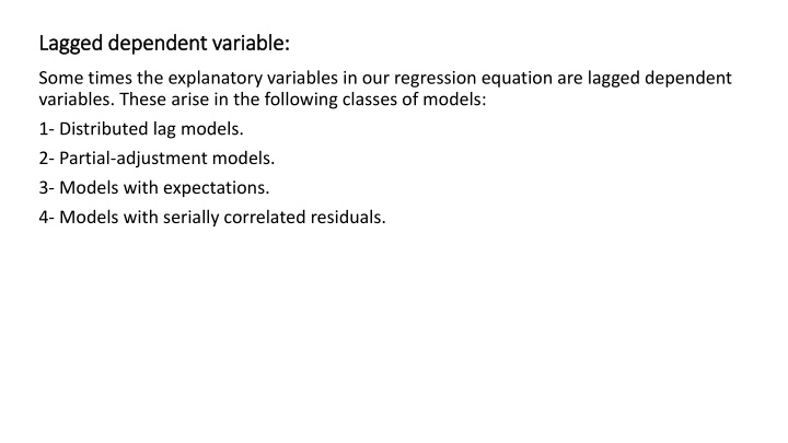
Lagged dependent variable: Lagged dependent variable: Some times the explanatory variables in our regression equation are lagged dependent variables. These arise in the following classes of models: 1- Distributed lag models. 2- Partial-adjustment models. 3- Models with expectations. 4- Models with serially correlated residuals.
1- Distributed lag models. Suppose that the current consumption ??depend on the current income ?? and on the incomes of the past (k) periods (?? 1, ?? 2, ?? 3, , ?? ?) , so we can write the model as following; ??= ?0??+ ?1?? 1+ ?2?? 2+ + ???? ? The above model called consumption function-distributed lag, because the lag with which income affects consumption is distributed over a number of periods. Because ??, ?? 1, ?? 2, ?? 3, , ?? ?, are very highly correlated, if we try to estimate equation (1), well get poor estimates of s , also we have loss one observation for each one lagged variable added to the function. For example if we start with 40 observations and use 15 lagged y s , we have only 25 observations to work with and 15 coefficients to estimate. 1
To solve this problem, Koyck suggested that s are successively diminish over time, that we assume that the ??to decline geometrically, i.e. we assumed ; ??= ???0 , j=1,2,3, and 0 < < 1 that is mean; ?1= ??0, ?2= ?2?0 , ?3= ?3?0, so that the smaller the value of the faster the decline and the smaller the lag between income and consumption. According to Koyck assumption, equation (1) becomes; ??= ?0??+ ?0??? 1+ ?0?2?? 2+ ?0?3?? 3+ from equation (2) we have; ?? 1= ?0??? 1+ ?0?2?? 2+ ?0?3?? 3+ 2 3
by subtracting eq.2 from eq.1 we get; ?? ??? 1= ?0?? And so we have; ??= ?0??+ ??? 1 Equation (4) represent a regression equation with lagged dependent variable as an explanatory variable, so we estimate a regression equation of ??on ??and ?? 1, and which give us estimates of ?0and , and then from these estimates we can obtain estimate for all ??. For example, consider the following estimated regression equation; ??= 5.2607 + 0.695??+ 0.231?? 1 from this estimated regression equation we have; ?0= 0.695 , ? = 0.231 from these estimates we can get the estimated regression model of the relationship between consumption and income, which is; ??= ???????? + 0.695??+ (0.695)(0.231)?? 1+ (0.695) 0.2312?? 2+ (0.695))(0.231)3?? 3+ ??= ???????? + 0.695??+ 0.161?? 1+ 0.037?? 2+ 0.008?? 3+ 0.002?? 4 The other coefficient are smaller, so we ignore them. 4
The estimated model can be explained as following; 1- the short-run marginal propensity to consume is equal to ( 0.695 ). 2- the long-run marginal propensity to consume is equal to; 0.695+0.161+0.037+0.008+0.002=0.903 which can also obtain as the sum of the following infinite series; 0.695 1 0.231= 0.903 0.695[1+0.231+(0.231)2+ (0.231)3+ ] = 3- increasing one unit in the income in time t lead to change the consume with amount ( 0.695 ). 4- increasing one unit in the income in time t+1 lead to change the consume with amount ( 0.161 ). 5- increasing one unit in the income in time t+2 lead to change the consume with amount ( 0.037). and so on. The most prominent case in distributed lag model is that the mean effect of the explanatory variable on the response variable do not limited to the current time t , but it distributed over time t . But how far we get back in time, it s mean the determination of the value of (k), and this what Koyck solved by his suggestion.
2 2- - Partial Partial- -Adjustment Model: Adjustment Model: The partial-adjustment model says that the actual change is only a fraction of the desired change. Let explain this model by the following two cases study: The first case study: suppose a firm anticipates some change in the demand for it s product, and to do that , it has to adjust it s productive capacity or say capital stock ( ??) , but it can not do this immediately. Let ( ?? ) be the desired capital stock, then (?? ?? 1) is the desired change. And ( ?? ?? 1) is the actual change. According to the partial-adjustment model, we have; ?? ?? 1= ?(?? ?? 1) Where ; 0 < < 1 Also suppose that the desired capital stock ( ?? ) is a function of sales ( ??), so that we have ; ?? = ? + ??? . 2 1
Combining eq.1 and eq.2 , we get; ?? ?? 1= ?(? + ??? ?? 1) So , ??= ?? + ????+ (1 ?)?? 1 Eq.3 can be written as following; ??= ?0+ ?1??+ ?2?? 1+ ?? Where; ?0= ?? eq.4 is a regression model with lagged dependent variable as an explanatory variable. Thus we estimate a regression equation of ??on ??and ?? 1, to get ( ?0, ?1, ?2), and from these estimated parameters we get the estimate of the eq.3 parameters; 3 . 4 , ?1= ?? , ?2= (1 ?) ?1 ?0 ? = 1 ?2 , ? = , ? = (1 ?2) (1 ?2)
The second case study: Let ?? be the desired consumption in period t , and suppose it is proportional to income ??that is; ?? = ??? 5 Also let the actual change in consumption ( ?? ?? 1) be a fraction of the desire change (?? ?? 1) That is ; ?? ?? 1= ?(?? ?? 1) 6 Combining eq.5 and eq.6 , we get; ?? ?? 1= ?(??? ?? 1) So, ??= ????+ (1 ?)?? 1 Which can be written as; 7 8 9 ??= ?1??+ ?2?? 1+ ?? Where; ?1= ?? , ?2= 1 ? eq.9 is a regression model with lagged dependent variable as an explanatory variable. Thus we estimate a regression equation of ??on ??and ?? 1, to get ( ?1, ?2), and from these estimated parameters we get the estimate of the eq.8 parameters;
?1 ? = 1 ?2 , ? = (1 ?2) It is easily seen that eq.8 is indistinguishable from eq.4 in Distributed lag models, thus when we estimate a regression equation of ??on ??and ?? 1, we can not tell whether this is a consequence of a Partial-Adjustment Model or a Distributed lag model.
3- Models with serially correlated error: Suppose we have the following model ; ??= ???+ ?? 1 And the residuals ??are not independent (serially correlated ), which follow the relationship ( ??= ??? 1+ ??) , where (??~??(0,?2), then we have; ?? ??? 1= ? ?? ??? 1 + ?? ??? 1 ??= ??? 1+ ??? ???? 1+ ?? Model (3) means that we have to estimate a regression equation of ??on ??, ?? 1( lagged dependent variable ), and ?? 1(lagged explanatory variable), note that there is a restriction on the coefficients of that model which is; coefficient of ?? 1= -(coefficient of ??)(coefficient of ?? 1) Hence this regression model must estimated by using one of the following methods: 1- nonlinear-least squares method. 2- search procedure on . 3- two-steps procedure. 2 3
The two-steps procedure: This method includes the following steps: 1- Estimate regression equation(3) with no restrictions, and estimate ( the coefficient of ?? 1) as ? . 2- using ? to transform the data as following: ?? = ?? ??? 1 ?? = ?? ??? 1 3- Estimate a regression equation of ?? on ?? ,that is mean estimate the following regression equation to get the estimated value of ; ?? = ?? + ?? Note: this procedure used in treating the autocorrelation problem. Note that eq.3 is similar to eq.4 in Distributed lag models, and also similar to eq.8 in Partial- Adjustment Model.