Laplace Transform Definitions and Results
Explore the Laplace transform definitions and results, including its properties and applications. Learn about transforming functions using Laplace transforms and understand the fundamental principles behind this powerful mathematical tool.

Download Presentation

Please find below an Image/Link to download the presentation.
The content on the website is provided AS IS for your information and personal use only. It may not be sold, licensed, or shared on other websites without obtaining consent from the author. If you encounter any issues during the download, it is possible that the publisher has removed the file from their server.
You are allowed to download the files provided on this website for personal or commercial use, subject to the condition that they are used lawfully. All files are the property of their respective owners.
The content on the website is provided AS IS for your information and personal use only. It may not be sold, licensed, or shared on other websites without obtaining consent from the author.
E N D
Presentation Transcript
LAPLACE LAPLACE TRANSFORMS TRANSFORMS
DEFINITION If a function f(t) is defined for all positive values of the variable 0 st ( ) e f t dt t and if exists and is equal to F(s) , then F(s) is called the Laplace transform of f(t) and is denoted by the symbol L{f(t)}. Hence The operator L that transform f(t) into 0 = = st { ( )} ( ) ( ). L f t e f t dt F s F(s) is called the Laplace transform operator.
RESULTS RESULTS
L{f(t)+g(t)} = L{f(t)}+L{g(t)} (i) we have L{f(t)+g(t)} = 0 + st [ ( ) ( )] e f t g t dt 0 + st st ( ) ( ) e f t dt e g t dt = 0 = L{f(t)}+L{g(t)}.
(ii) L{cf(t)} = cL{f(t)} , where c is a constant. 0 we have L{cf(t)} = st ( dt t ) e cf = 0 st ( dt t ) c e f = cL{f(t)}.
(iii) L{f(t)} =sL{f(t)}- f(0). 0 st ( ' ) e f t dt we have L{f (t)} = = (on integration by parts) 0 0 st st ( )[ ] ( )( ) f t e f t s e dt 0 = + st ) 0 ( ( ) f s e f t dt = sL{f(t)}-f(0) .
(iv) ( ' ' { t f L = 2 )} { ( )} ) 0 ( 0 ( ' ). s L f t sf f L{f (t)} = L{F (t)} where F(t)=f (t) = sL{F(t)}-F(0) = sL{f (t)}-f (0) = s[sL{f(t)}-f(0)]-f (0) 2s = L{f(t)}-sf(0)-f (0).
(v) By extending the previous result , we get = 1 1 2 1 n n n n n n { ( )} { ( )} ) 0 ( ) 0 ( 0 ( ' )...... 0 ( ). L f t s L f t s f s f s f f (vi) If L{f(t)} = F(s) (a) lim t = ( ) lim s ( ). f t sF s 0 (b) = lim t ( ) lim s ( ). f t sF s 0
(vii) L 1 = at ( ) e + s a 0 = at st at ( ) L e e e dt 0 + = ( ) s a e dt + ( ) s a t e = + ( ) s a 0 1 = s + a 1 Similarly = at ( ) L e s a
(viii) L s + = (cos ) . at 2 2 s a 0 = st (cos ) cos . L at e atdt + st ( cos s sin ) e s at a at = + 2 2 a 0 s + = . 2 2 s a (ix) similarly a + = (sin ) . L at 2 2 s a
(x) ) ( t L + ( ) 1 1 + n = n . n s 0 = n st n We have . ( t L ) e t dt n 1 s x by putting st=x. = n x ( ) . L t e dx s 0 1 n . 0 = n x x e dx + 1 s + ( ) 1 1 + n = . n s
Thank you Prepared by D.PHILOMINE JEEVITHA Department of Mathematics St.Joseph s college trichy


+g(t)} = L{f(t)}+L{g(t)}")
 L{cf(t)} = cL{f(t)} , where c is a constant.")
 L{f’(t)} =sL{f(t)}- f(0).")
")
 By extending the previous result , we get")
")
")
")