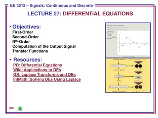
Laplace Transforms for Solving Initial Value Problems
Laplace transforms are introduced as a powerful mathematical tool to solve initial value problems in the realm of classical mechanics and mathematical methods. The lecture covers the definition of Laplace transforms, their applicability in solving differential equations, and techniques involving complex variables and contour integrals.

Download Presentation

Please find below an Image/Link to download the presentation.
The content on the website is provided AS IS for your information and personal use only. It may not be sold, licensed, or shared on other websites without obtaining consent from the author.If you encounter any issues during the download, it is possible that the publisher has removed the file from their server.
You are allowed to download the files provided on this website for personal or commercial use, subject to the condition that they are used lawfully. All files are the property of their respective owners.
The content on the website is provided AS IS for your information and personal use only. It may not be sold, licensed, or shared on other websites without obtaining consent from the author.
E N D
Presentation Transcript
PHY 711 Classical Mechanics and Mathematical Methods 10-10:50 AM MWF in Olin 103 Notes for Lecture 24: Chap. 7 & App. A-D (F&W) Generalization of the one dimensional wave equation various mathematical problems and techniques including: 1. Laplace transforms 2. Complex variables 3. Contour integrals 10/23/2023 PHY 711 Fall 2023-- Lecture 24 1
10/23/2023 PHY 711 Fall 2023-- Lecture 24 2
10/23/2023 PHY 711 Fall 2023-- Lecture 24 3
Last time, we introduced the Fourier Transform -- Definition of Fourier Transform for a function ( ): f t i t = ( ) F ( ) f t d e Note that: = Backward transform: i t co s( ) sin( ) e t i t 1 i t = ) F( dt f(t) e 2 In this lecture, we will discuss a similar concept the Laplace Transform. i p 10/23/2023 PHY 711 Fall 2023-- Lecture 24 4
A brief introduction to Laplace transforms -- Laplace transforms are particularly useful in solving initial value problems. The Lapace transform of the functi on ( ) is defined: x ( ) x dx px ( ) p L e ( ) x 0 Assuming that ( ) is identities can be shown: wel l -behaved in the interval 0 , the following x x ( ) x dx d + px ( ) p = (0) ( ) p L e dx pL ( )/ x ( ) x d dx 0 and 2 ( ) x (0) dx d d + 2 px ( ) p = (0) ( ) p L e dx p p L ( ) x 2 2 ( )/ x 2 d dx dx 0 10/23/2023 PHY 711 Fall 2023-- Lecture 24 5
Some details (integrating by parts)-- R e all c ( ) x dx px ( ) p L e ( ) x 0 Then: ( ) x dx d d dx ( ) p e ( ) x dx + ( ) x dx px px px ( ) p = L e dx e ( )/ x dx d 0 0 0 = + (0) ( ) p pL ( ) x 10/23/2023 PHY 711 Fall 2023-- Lecture 24 6
10/23/2023 PHY 711 Fall 2023-- Lecture 24 7
We can check that this a solution to the differential equation = 2 d dx d dx = = x for (0) 0 and (0) 0 F e 0 2 10/23/2023 PHY 711 Fall 2023-- Lecture 24 8
Using Laplace transform solve to s equation : 2 0 d x d ( ) = ) 0 ( = = wit L 1 ( ) sin h , 0 0 x F 0 2 dx L dx F ( ) p = L 0 2 ( ) + + 2 2 1 p p L / 1 1 L = F ( ) 0 + 2 2 2 1 p / 1 L + 2 p L a ( ) at 0 F = pt Note that : sin e dt + 2 2 a p x ( ) x = 0 sin sin( ) x ( ) 2 L L / 1 L 10/23/2023 PHY 711 Fall 2023-- Lecture 24 9
Table of Laplace transforms https://www.dartmouth.edu/~sullivan/22files/New%20Laplace%20Transform%20Table.pdf 10/23/2023 PHY 711 Fall 2023-- Lecture 24 10
Inverse Laplace transform : In order to evaluate these integrals, we need to use complex analysis. ( ) p L ( ) t 0 = pt e dt + i 1 ( ) t ( )dp p L = pt e 1 2 i i + + i i 1 ( ) p dp ( ) u du 0 = pt pt pu L Check: 2 e e dp e 2 i i + i i i 1 1 ( ) u du ( ) u du ( ) ( ) ( ) t u p t u is t u = e dp e e ids 2 2 i i 0 0 i ( ) 1 ( ) u du e ( ) if 0 otherwise ( ) ( ) t u = 2 i t u 2 i 0 0 t t = 10/23/2023 PHY 711 Fall 2023-- Lecture 24 11
In general to calculate inverse Laplace transforms, we need to introduce concepts of complex numbers and contour integration Introduction to complex variables 1. Basic properties 2. Notion of an analytic complex function 3. Cauchy integral theory 4. Analytic functions and functions with poles 5. Evaluating integrals of functions in the complex plane 10/23/2023 PHY 711 Fall 2023-- Lecture 24 12
Complex numbers = + 2 1 Define 1 i i = z x iy ( )( ) 2 = = + = + 2 2 * z zz x iy x i y x y Polar representation sin cos i + ( ) = = i z e Functions of complex variables ( ) f z = ( ) ( ) ( ) f z ( ) f z + + ( , ) u x y ( , ) iv x y i Derivatives: Cauchy-Riemann equations ( ) f z x ( ) u z x ( ) v z x f z x ( ) f z i y ( ) u z i y u z x ( ) v z i y ( ) v z y ( ) u z y = + = + = i i i ( ) ( ) f z i y ( ) ( ) v z y ( ) v z x ( ) u z y df dz = = = Argue that = and 10/23/2023 PHY 711 Fall 2023-- Lecture 24 13
Analytic function ( ) is analytic if it is: continuous single valued its first derivative satisfies Cauchy-Rieman conditions f z Examples of analytic functions + = = + z x i y x x cos( ) = ( x = sin( ) v x ) 2 + e e e y ie y u x v y u y = = = x x cos( ) sin( ) e y e y ( ) 2 = x iy + + 2 2 2 ( , ) ( , ) z y ixy u x y iv x y u x v y v x u y = = = = 2 2 x y 10/23/2023 PHY 711 Fall 2023-- Lecture 24 14
Examples of non-analytic functions + = + = 2 ie i i i n Note that ln for any integer z e n ( ) = + ln 2 z n ln is not analytic because it is multivalued z n is not analytic for non-integer because it is multivalued = 2 i i z e e z 1 z = = Behavior of ( ) about the point 0: f z z n For an integer , consider n = 2 2 0 1 1 n n i 1 z e i d = = = 1 (1 ) n i n dz e id n n in 2 i e 0 0 10/23/2023 PHY 711 Fall 2023-- Lecture 24 15
1 z = = Behavior of ( ) about the point 0: f z z n For an integer , consider n = 2 2 0 1 1 n n i 1 z e i d = = = 1 (1 ) n i n dz e id n n in 2 i e 0 0 This observation helps us to focus on a special kind of singularity called a "pole" ( ) g z z = p z For ( ) in th f z e vicinity o f : ( ) z z f z p p dz = = = ig z Therefore: ( ) f z dz 0 or ( ) ( ) 2 ( ) f z dz g z p p z z p Integration does not include zp Integration does include zp 10/23/2023 PHY 711 Fall 2023-- Lecture 24 16
( ) = ( ) z 2 Res ( ) f dz i f z p ( ) z = p y C No contribution z p ( ) ( ) f z z Res ( ) ( ) f z p ( ) f z 2 Res i z p z p p ( ) z = x z p z p C 10/23/2023 PHY 711 Fall 2023-- Lecture 24 17
General formula for determining residue: ( ) Res ( z ) f z ( ) h z p Suppose that in the neighborhood of , ( ) z f z ( ) p m z z z z z p p p ( ) m Since ( ) ( ) is analytic near f z , we can make Taylor exansion ( ... ( 1)! m a h z z z z p p ) 1 m z z 1 m ( dz ) ( ) dh z d h z ( ) p + + + + p p ab u o t : ( ) z ( ) .... z h h z z z p p p 1 m dz ) ( ( ) m 1 m ( ) d z z f z 1 ( ) p lim z = Res ( ) f z p 1 m ( 1)! m dz z p In the following examples m=1 10/23/2023 PHY 711 Fall 2023-- Lecture 24 18
2 2 2 x + x + z + = + = 0 dx dx dz Example: 4 4 4 1 1 1 x x z Im(z) Re(z) ( )( ( )( )( ) + = 4 /4 3 /4 /4 3 /4 i i i i 1 z z e z e z e z e Note: m=1 ) 2 z + ( ) ( ) = = + = /4 3 /4 i i 2 Res Res dz i z e z e p p 4 1 z /4 3 /4 i i e e ( ) ( ) = = = = /4 3 /4 i i Res Res z e z e p p 4 4 i i 2 /4 3 /4 i i 1 2 1 2 1 2 1 2 z + e e = = + + = 2 dz i i i 4 1 4 4 2 z i i 2 10/23/2023 PHY 711 Fall 2023-- Lecture 24 19
Some details: = = i i Note that: 1 = e e 2 z + = 3 /4 /4 /4 i i i i e e e = ( ) f z 4 1 z ( /4 ) 2 / 4 i e ( ) = = /4 i Res ( f z e ( )( )( ) /4 3 /4 /4 /4 3 /4 i i i i i i e e e e e e /2 i e = ( )( e )( ) + + /4 /4 /4 / 4 /4 / 4 i i i i i i e e e e e e / 4 / 4 i i e = =2 ( ) ( ) 4 i i i Question Could we have chosen the contour in the lower half plane? a. Yes b. No 10/23/2023 PHY 711 Fall 2023-- Lecture 24 20
I = Another example: iax iaz cos( + + ) 1 2 1 2 ax e e = = dx dx dz + + + + + Note: m=1 4 2 4 2 4 2 4 5 1 4 5 1 4 5 1 x x x x z z 0 4 )( )( )( ) ( + = + + 4 2 5 1 4 i i z z z i z z i z 2 2 Im(z) Re(z) ( ) ( ) ( ) = = + = 2 Res R es i I i z i z p p 2 10/23/2023 PHY 711 Fall 2023-- Lecture 24 21
iaz cos( + ) 1 2 ax e = dx dz + + + 4 2 4 2 4 5 1 4 5 1 x x z z 0 ( ) ( ) ( ) = + = =2 Res Res i i z i z p p 2 ( ) + /2 a a = 2 e e 6 Question Could we have chosen the contour in the lower half plane? a. Yes b. No Note that for 0 and 0 = a z I iaz az ia z in the lower half pla e: n e e e R I 10/23/2023 PHY 711 Fall 2023-- Lecture 24 22
sin + x x kxdx a I = for 0 and 0 k a Another example: 2 2 ikx ikz sin + + 1 i 1 i x x kx xe ze = = dx dx dz + + 2 2 2 2 2 2 a = x a z a ( )( ) + 2 2 z a z ia z ia Im(z) ia Re(z) ( ) ( ) = = = ka 2 R s e I i z ia e p 10/30/2017 PHY 711 Fall 2017 -- Lecture 25 23 10/23/2023 PHY 711 Fall 2023-- Lecture 24 23
Some details -- ikx ikz sin + + 1 i 1 i x x kx xe ze = = dx dx d z + + 2 2 2 2 2 2 a = x a z a ( )( ) z ia + 2 2 z a z ia ikz ikz 1 i 1lim ( z i ze ze = z ia 2 ) dz i + + 2 2 2 2 z a z a ia ka 1 i i ae = ka = 2 i e 2 ia 10/23/2023 PHY 711 Fall 2023-- Lecture 24 24
From the Drude model of dielectric response -- 2 p i e = ( ) where , , an d are positive constan t s G d 0 p 2 0 2 2 i Upper hemisphere: e Converges for + = + = i ix y e z x iy Im(z) 0 i i Re(z) 0 0 2 2 Lower hemisphere: e Converges for 2 = = i ix y e z x iy 2 0 0 4 0 10/23/2023 PHY 711 Fall 2023-- Lecture 24 25
From the Drude model of dielectric response -- contin ued -- 2 p i e = ( ) where , , a nd are positive c o nstan ts G d 0 p 2 0 2 2 i 0 s for 0 = 2 p ( ) G in /2 for 0 0 e 0 10/23/2023 PHY 711 Fall 2023-- Lecture 24 26


--")