Learn the Basics of STATA Software for Data Analysis
Explore an introduction to STATA software, covering data description, graph creation, software structure, working with files, and organizing data effectively. Get started with this comprehensive tutorial.

Download Presentation

Please find below an Image/Link to download the presentation.
The content on the website is provided AS IS for your information and personal use only. It may not be sold, licensed, or shared on other websites without obtaining consent from the author. If you encounter any issues during the download, it is possible that the publisher has removed the file from their server.
You are allowed to download the files provided on this website for personal or commercial use, subject to the condition that they are used lawfully. All files are the property of their respective owners.
The content on the website is provided AS IS for your information and personal use only. It may not be sold, licensed, or shared on other websites without obtaining consent from the author.
E N D
Presentation Transcript
STATA I: An Introduction Into the Basics Prof. Dr. Herbert Br cker University of Bamberg Seminar Migration and the Labour Market Session 3 May 21, 2015
Contents 1 2 3 4 5 6 7 8 9 10 Describe your data 11 Making graphs The STATA Software package The Structure of STATA: Three files Getting started The STATA Menues The General Structure of STATA Working with DO FILES Generarting Dummy Variables The log transformation Organize your data with globals
1 STATA SOFTWARE PACKAGE Download Software: http://download.stata.com/download/ Look for Password which matches your username (from the list I mailed) Username: Password: Important: Register always under OTTO-FRIEDRICH-UNIVERSIT T, Bamberg
2 Structure of STATA: Three files 1. The DATA file (.dta) where you have your data. You can watch you data with the DATA BROWSER and edit your data with the DATA EDITOR 2. The DO file (.do) where you run and save your commands of any session. Very useful (i) to organise your data set, (ii) to see what you have done in the last session, (iii) to replicate what you have done in last session, (iv) to exchange work with your collaborators. You write and run your commands with the DO FILE EDITOR
2 Structure of STATA: Three files 3. The LOG file (.log) which automatically reports all things which you have done during your session. Is automatically saved after your session. Useful if something goes wrong.
3 Getting started: the STATA empty window
3 Getting started: The STATA empty window The main window: shows commands, output and messages which arrive during your session
3 Getting started: The STATA empty window The main window: shows commands, output and messages which arrive during your session The command window: here you can type your commands
3 Getting started: The STATA empty window The main window: shows commands, output and messages which arrive during your session The variables window: Shows variables of your dataset The command window: here you can type your commands
3 Getting started: The STATA empty window The review window reports your previous commands The main window: shows commands, output and messages which arrive during your session The variables window: Shows variables of your dataset The command window: here you can type your commands
3 Getting started: the windows after data loading Reports commands (one in this case) Reports result of commands List of variables
3 Getting started In principle, you can start your STATA session by (i) loading your data set and (ii) typing your commands in the command window. It is however recommended to use the DO FILE EDITOR right from the beginning. But let s look at the STATA menues first.
4 The STATA Menues The data path The do file editor The data editor The data browser The variables manager The help menue For watching your data and changing your data by hand you need the DATA BROWSER and the DATA EDITOR. For starting and running your DO files you need the DO FILE EDITOR. The other menues are not relevant for the beginning.
4 The STATA Menues: The DATA EDITOR/BROWSER The difference between the data browser and the data editor is that you can manipulate data in the editor and only watch them in the browser.
4 The STATA Menues: The DATA EDITOR/BROWSER STRING variable NUMERICAL variable You have two types of variables: NUMERICAL variables (black) and so-called STRING variables (red) (e.g. text). STATA can identify STRING variables, but you cannot do numerical operations with them.
4 The STATA Menues: The DATA EDITOR/BROWSER HINT: You can transfer data e.g. from an EXCEL file into a STATA file by copy and paste (STRG C + STRG V) and vice versa in the data editor. But you have to be careful that you EXCEL is run in English, otherwise your data might be read as STRING variables by STATA. Better: Use the import excel command.
The Grammar of STATA 5 General Structure of STATA commands [prefix :] command [varlist] [if] [in] [weight] [, options]
General structure of STATA 5 We will concentrate on: [prefix :] command [varlist] [if] [in] [weight] [, options]
5 General structure of STATA We will concentrate on: [prefix :] command [varlist] [if] [in] [weight] [, options] What you want to do?
General structure of STATA 5 There are two types of variables (data): numerical variables, e.g.: 0, 1, 501, 0.5, -12 etc. string variables, e.g.: no voc train , male, female etc. How to deal with the data types: Numerical variables: you can do all mathematical operations, e.g. var1 + var2, var1/var2, var1*var2 etc. String variables: You have to use quotation marks for identification, e.g. var1 = 1 if sex == female
6 Working with DO FILES The standard approach is to start your work with a DO FILE Click on the DO FILE editor button after starting STATA Load an existing DO FILE or start a new one Start the DO FILE with a command to load your data, e.g. use path\data.dta , clear or, more specifically, with Use"C:\Users\Herbert\Documents\STATA\Projectseminar_2014\Germany\DE.dta", clear
Open your DO FILE editor The do file editor After starting STATA click on the DO FILE editor button
How does a DO FILE look like Descriptions of what you have done in stars * Commands
The DO FILE menue Clicking this button runs the entire DO FILE (not recommended) Clicking this button runs a selection of marked commands (recommended) Note: STATA stops the DO File execution after the first mistake in your commands. That makes it advisable to proceed step by step.
6 Data organization: General issues The basis for all what you do is your Do-File which you open in all sessions first Work with a small data set and do the generation of all additional variables based on your Do-File in the beginning of each session. Save only the small dataset. That is efficient from the data management side and reduces the risk that you delete/change important variables which you cannot restore. Change somewhere a save version of your dataset. Use log filed that you can see in case of a problem what you have actually done. You seldomly look at it, but you might miss it in an important case
6 Step 1: Starting your session Open a Do-file with the Do-File editor or load an existing one The clear command clears data from your memory The cap clear matrix command clears matrix from your memory (if there is one) Note: the capture or cap command is useful: is signals STATA to use the command only if it is needed The cap log close command closes the log file if there is one open The set more off command is not necessary, but you can proceed faster since Stata always stops otherwise if the command lines exceed your screen
6 Step 1: Starting your session (cont.) The glo path C: . defines a path where you want to work, e.g. where your have your data The cd path command changes the directory to the path you have defined before The cap log using log\de.log, replace command opens a log file and replaces an existing one if there is one Note: Your have create the folder for your log file before. Of course you can also save your log filed in the main folder e.g. by typing cap log using de.log, replace
6 Step 2: Loading your data If you have already a STATA data file: The use command loads the data the path\data\DE.dta, clear provides STATA the information on the path where to find the data and the name of the data file (e.g. DE.dta) the clear command after the comma clears the memory, which is needed if you have used other data sets before
6 Step 2: Loading your data (cont.) If you have to import data e.g. from an Excel file: Use the import excel using path\data\de.xlsx, firstrow command the import excel tells STATA that it has to import a file with a different data format, in this case excel using path\data\de.xlsx tells data where to find the data and the file name The option after the comma ,firstrow tells STATA that it has to treat the first row of the Excel sheet as the names (labels) of the variables. Otherwise it thinks it are data and you end up in a mess.
Loading your data (I/II) 1. Write the command use path\XXX.dta , clear 2. Mark the line and run the command by clicking the execution button
6 Step 3: Manipulating your data (I) Your can generate new variables and replace existing one E.g. generate a numerical variable by using the information from a STRING variable gen ed = . generates the variable ed with missing values in the first place In the next step you can replace the values of this variables by using replace ed = 1 if education == no voc training Which assigns the varianble a vale of 1 if the person/group has no vocational training
6 Step 3: Manipulating your data (II) replace ed = 1 if education == no voc training replace tells STATA to replace the values of the variable, in this case of the ed variable by 1 the if option tells STATA under which conditions, note that you have to use double equality sign (==) after the if option The double signs in no vocational training tells STATA that we have a STRING variable Then repeat this until all values of your variable are filled
6 Step 3: Manipulating your data (III) Useful operators in STATA: + - * / ln exp add subtract multiply divide transform into natural log transform into exponential value
7 GENERATE Dummy Variables Borjas (2003) model Why dummy variables How to create dummy variables Advanced techniques to create dummy variables
Recall the Borjas (2003)-Modell where yijtis the dependent variable (e.g. log wage, unemployment rate) siis an education dummy xjis an education dummy pijis a time dummy plus many interaction dummies Thus, we have to create quite a bunch of dummmy variables. But, in the first place, what are dummy variables doing?
7 Generate dummy variables: how to do Generating DUMMY variables Use the gen command, e.g. gen Ded1 = 0 This creates a variable consisting only of zeros Then use the replace command, e.g. replace Ded1 = 1 if ed == 1 This replaces the zeros with 1 if the variables ed1 has a values of 1.
7 Dummy variables Another example for generating dummy variables: Use the gen command, e.g. gen Dt1 = 0 This creates a variable consisting only of zeros Then use the replace command, e.g. Dt1 = 1 if year == 1991 This replaces the zeros with 1 if the year variable has a values of 1991 Note: The STATA syntax requires that you have to use after an if command always a double == for the definition of the value
7 Generating dummy variables: advanced techniques Creating series of dummy variables if it is too cumbersome to create them individually, e.g. in case of interaction dummies Syntax: forvalues i = 1/3 { forvalues j = 1/4{ gen D_ed`i *D_ex`j } } i.e. for each value I = 1,2,3 and each value j = 1,2,3,4 you generate an interaction dummy by multiplying the dummy variables for education and experience. Take care of the {}!
8 Log transformation Transforming variables into log variables Syntax: gen ln_wijt = ln wijt By using again the gen command you can transform the wage variable wijt into the natural logarithm of the wage by applying the ln operator
9 Organize your data with globals It is not convenient if you have to work with too many variables, e.g. 200 dummy variables (that is cumbersome to type some by hand) You can define globals, which comprise many variables Syntax: glo [name of global [list of variables] glo Di Ded_1 Ded_2 D_ed3 i.e the global Di consists of the variables Ded_1 Ded_2 and Ded_3 If you want to use the global later you have to type $[globalname], i.e. $Di
10 Describe your data (I/II) Any econometric analysis requires in the first step that you provide descriptive statistics to the reader. This helps to understand what s going on This can be easily done with the sum command sum [variable name(s)] sum LHijt LFijt wijt ln_wijt The sum command creates a table with the complete descriptive statistics, i.e. observations, mean, standard deviation, minimum, maximum


")
")


-Modell")


")