Learning Mixtures of Linear Regressions with Nearly Optimal Complexity
"This presentation discusses mixtures of linear regressions, a widely studied topic in both theory and practice. It covers the basics of Mixture of Linear Regressions (MLR) models, their applications, and the goal of learning hidden parameters in the regressions. The work explores classical models, theoretical analyses, benchmark algorithms, and new algorithm design in the realm of non-convex optimization. The content dives into problem definitions, simplified settings with constant numbers of components, and general assumptions addressed by current research in the field."

Download Presentation

Please find below an Image/Link to download the presentation.
The content on the website is provided AS IS for your information and personal use only. It may not be sold, licensed, or shared on other websites without obtaining consent from the author.If you encounter any issues during the download, it is possible that the publisher has removed the file from their server.
You are allowed to download the files provided on this website for personal or commercial use, subject to the condition that they are used lawfully. All files are the property of their respective owners.
The content on the website is provided AS IS for your information and personal use only. It may not be sold, licensed, or shared on other websites without obtaining consent from the author.
E N D
Presentation Transcript
1 Learning Mixtures of Linear Regressions with Nearly Optimal Complexity Yingyu Liang@UW-Madison Joint work with Yuanzhi Li@Princeton, to appear in COLT 18
2 Mixture Models General way to build sophisticated models from simple models
3 Mixture Models General way to build sophisticated models from simple models Widely studied in theory and practice Mixture of Gaussians Topic Modelling
4 Mixture Models General way to build sophisticated models from simple models Widely studied in theory and practice Mostly about unsupervised learning This work: a prototypical mixture model in supervised learning, Mixture of Linear Regressions (MLR)
5 Mixture of Linear Regressions (MLR) Given: a mixture of data points from ? unknown linear regression components (without knowing which point belong to which component) Goal: learn the hidden parameters in the ? regressions Mixed Data
6 Mixture of Linear Regressions (MLR) Given: a mixture of data points from ? unknown linear regression components (without knowing which point belong to which component) Goal: learn the hidden parameters in the ? regressions Classical model dates back to (De Veaux, 1989) Simple yet effective in capturing non-linearity Theoretical topic for analyzing benchmark algorithms (Chaganty and Liang, 2013; Klusowski et al., 2017) or designing new algorithms (Chen et al., 2014; Zhong et al., 2016) for nonconvex optimization
7 Problem Definition Suppose ? linear regression components Component ? has regression parameter ?? ??, data distribution ?? over ??and data fraction ?? 0, where ???= 1 Data point ?,? generated iid as follows: Sample component id ?~ multinomial({??}) Generate input ? ~ ?? Generate regression response ? = ??,? Problem of Learning MLR Given: dataset ??,??,1 ? ? Goal: learn {??,1 ? ?}
8 A Simplified Setting Constant number of components, e.g., ? = 5 Gaussian: ??= ?(0, ? Nonvanishing component: ?? 2), and ? ? 2? 1 10 1 10 Separation: ?? 2 1 and ?? ?? 2 Our work can handle much more general assumptions
9 Main Result for the Simplified Setting Global convergence, recovery to any accuracy Sample/Computational complexity has nearly optimal dependence on the dimension
12 Comparison with Existing Work Our assumptions are cleaner and more general Better sample/computational complexity
13 Algorithm/Analysis Overview Let s focus on learning one of the regression weights Once learned, can remove points from that component and repeat Two phases for learning one weight Moment Descent to get a warm start Method of Moments for incremental update Gradient Descent to get an accurate solution Specific designed concave objective function
14 Warm Start I: Overview Maintain ?? at iteration ?, and update it by ??+1= ??+ ? ?? so that min { ??? ?? 2} gets smaller and smaller ?
15 Warm Start I: Overview Maintain ?? at iteration ?, and update it by ??+1= ??+ ? ?? so that min { ??? ?? 2} gets smaller and smaller ? First attempt: ?? ~ ?(0,?) is a random direction with prob >1/4, ?? is positively correlated with ?? ?? where ? = argmin? ??? ?? 2 Make progress!
16 Warm Start I: Overview Maintain ?? at iteration ?, and update it by ??+1= ??+ ? ?? so that min { ??? ?? 2} gets smaller and smaller ? First attempt: ?? ~ ?(0,?) is a random direction with prob >1/4, ?? is positively correlated with ?? ?? where ? = argmin? ??? ?? 2 Make progress! 1 ? progress per iteration But too slow: ?
17 Warm Start I: Overview Maintain ?? at iteration ?, and update it by ??+1= ??+ ? ?? so that min { ??? ?? 2} gets smaller and smaller ? Our method: ?? ~ ?(0,?? ) where ? ?? ? and its span contains a vector correlated with ?? ?? If well correlated then can make fast progress How to get such ??
18 Warm Start II: Method of Moments Use Method of Moments to get a good ? When all ?= ?, ? ? ??,? ?? ? + ?? where span of ? ?? ? is the subspace by (?? ??) s 1 ? progress per iteration Using this, leads to
19 Warm Start II: Method of Moments Use Method of Moments to get a good ? When all ?= ?, ? ? ??,? ?? ? + ?? where span of ? ?? ? is the subspace by (?? ??) s 1 ? progress per iteration Using this, leads to However, this fails when ? s are different
20 Warm Start III: Method of Polynomials When ? s are different: also apply Method of Polynomials Compute 2??? ??? ? ??,? ?=0, ,? where ?? s are set such that terms related to (?? ??) s are preserved while other terms are cancelled
21 Warm Start III: Method of Polynomials When ? s are different: also apply Method of Polynomials Compute 2??? ??? ? ??,? ?=0, ,? where ?? s are set such that terms related to (?? ??) s are preserved while other terms are cancelled ?? s are set to be the coefficients of some polynomial carefully designed to satisfy the requirement
22 Gradient Descent from Warm Start ???? ? Given a warm start ???? gradient descent to minimize the function ? ? = ?[log(|? ?,? | + ?)] where ? is some parameter away from the truth, use Without ?, similar to the Gravitational allocation method With ?, ensure the smoothness of the function Prove the convergence by lower bounding ? ? ,?? ?
23 Conclusion Algorithm for learning Mixture of Linear Regressions in a quite general setting Achieves sample and computational complexity nearly optimal in the dimension Based on Moment Descent technique, which may be of independent interest