Leveraging AI for Improving Evapotranspiration Forecasting

NOAA Workshop on Leveraging AI in the Exploitation of Satellite Earth Observations and Numerical Weather Prediction for enhancing reference evapotranspiration forecasting in agriculture. Focus on improving NWP models, post-processing methods, and influencing factors for accurate ETo predictions. Utilizing FAO-56 Penman Monteith method for computation.

• NOAA
• AI
• Evapotranspiration
• Forecasting
• Agriculture

hauschild_r Follow

Uploaded on Mar 13, 2025 | 0 Views

Download Presentation

Please find below an Image/Link to download the presentation.

The content on the website is provided AS IS for your information and personal use only. It may not be sold, licensed, or shared on other websites without obtaining consent from the author.If you encounter any issues during the download, it is possible that the publisher has removed the file from their server.

You are allowed to download the files provided on this website for personal or commercial use, subject to the condition that they are used lawfully. All files are the property of their respective owners.

The content on the website is provided AS IS for your information and personal use only. It may not be sold, licensed, or shared on other websites without obtaining consent from the author.

Presentation Transcript

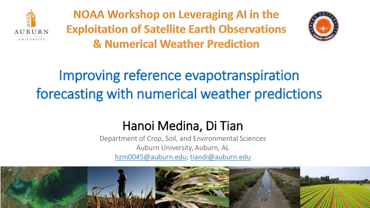
1. NOAA Workshop on Leveraging AI in the Exploitation of Satellite Earth Observations & Numerical Weather Prediction Improving reference evapotranspiration Improving reference evapotranspiration forecasting with numerical weather predictions forecasting with numerical weather predictions Hanoi Medina, Di Tian Hanoi Medina, Di Tian Department of Crop, Soil, and Environmental Sciences Auburn University, Auburn, AL hzm0045@auburn.edu; tiandi@auburn.edu

2. Evapotranspiration is the water lost through plant transpiration and soil and plant evaporation. Mass and energy balance on the earth surface Water and resource management in agriculture

3. Crop Reference evapotranspiration evapotranspiration Crop Reference Evapotranspiration Coefficients

4. Forecast outputs from numerical weather prediction (NWP) models are potentially useful for reference ETo forecasting. But usually have systematic errors Multi model ensembles Post-processing methods

5. We have been aimed to improve the NWP forecasts of ETo across the CONUS 1) The potential of single and multi-model forecasts 2) The performance of the ETo forecasts using no post- processing, compared with traditional and state of art post- processing schemes. 3) The influence factors such as lead-time, region, and the uncertainty of the individual weather variables.

6. They were computed using the FAO-56 Penman Monteith (Allen et al., 1998) 900 0.408 ?? ? + ? ? + 273?2 ?? ?? + ? 1 + 0.34?2 ??0= ?? is the net surface radiation at the crop surface [MJm 2day 1], ? is the soil heat flux density [MJm 2day 1], ? is the daily mean air temperature at 2 m height [ C], ?2 is the wind speed at 2 m height above ground [ms 1], ?? is the saturation vapor pressure [kPa], ?? is the actual vapor pressure [kPa], is the slope of the vapor pressure curve [kPa C 1] ? is the psychometric constant [kPa C 1].

7. Observations (https://www.ncdc.noaa.gov/crn/) daily measurements from 101 quality- controlled U.S. Climate Network (USCRN) weather stations were used as the observational reference. Reference Tmin, Tmax, Rs, RH, u, between May - August (2014 to 2016) The NCEI climate regions (NW (North West); WNC (West North Central), ENC (East North Central), NE (North East), C (Central), SE (South East), C (Central), S (South), SW (South West), W (West). The solid dots represent the USCRN stations used in this study. Forecasts http://www.ecmwf.int/en/forecasts/datasets/set perturbed ensemble forecasts The THORPEX Interactive Grand Global Ensemble TIGGE the Eur. Center Medium Range Weather Forecast (EC) the Nat. Centers for Environ. Pred. Global Forecast Sys. (NCEP) the United Kingdom Meteorological Office (MO)

8. Forecasts strategies Metrics Correlation RMSE EC, NCEP, MO single forecasts Deterministic Rank histograms Coverage Spread-skill CRPS BSS Reliability EC_MO multi-model forecasts EC_NCEP_MO Probabilistic Training period = 30 days Considering lower, middle and upper terciles

9. Comparing raw forecasts 1.6 1-day lead 7-day lead 1.4 RMSE (mm) 1.2 1 0.8 0.6 EC NCEP MO EC_MO EC_NCEP_MO Forecasting strategy Medina et al., 2018. Medium-range reference evapotranspiration forecasts for the contiguous United States based on multi-model numerical weather predictions. J. of Hydrol., 562, pp.502-517.

10. 2.0 2.0 2.0 1.5 1.5 1.5 1.0 1.0 1.0 2.0 0.5 0.5 0.5 2.0 2.0 2.0 1.5 0.0 0.0 0.0 1.5 1.5 -0.5 -0.5 1.5 -0.5 1.0 0.5 SW SW NE EC EC NCEP NCEP EC NCEP SE SE S W W NE NE ENC ENC NW NW C WNC WNC SE S S SW W ENC NW a) a) C C WNC 2.0 1.0 1.0 1.0 b) b) a) b) Rs u u u T RH RH RH Rs Rs T T 2.0 2.0 2.0 2.0 2.0 2.0 0.0 1.5 1.5 1.5 1.5 1.5 1.5 1.0 1.0 1.0 1.0 1.0 1.0 ME (mm) ME (mm) ME (mm) 1.5 -0.5 0.5 0.5 0.5 0.5 0.5 0.5 0.5 0.5 0.5 0.0 0.0 0.0 0.0 0.0 0.0 -0.5 -0.5 -0.5 -0.5 -0.5 -0.5 Comparing EC and NCEP raw forecasts EC SW W NE SW NE ENC NW C WNC NW NW -1.0 -1.0 -1.0 -1.0 -1.0 SE W W -1.0 SE SE WNC NCEP SE SW SW S ENC C 2.5 C NW C WNC SE S SW SW W W NE ENC NW C WNC SE S S SW SW SW W W W NE ENC NW NE ENC NW C WNC C WNC S SE W S NE NE W ENC ENC NE ENC NW ENC T C WNC NW Rs c) c) S NE ENC NW C WNC 1.0 SE SE S SE S S SW 2.5 2.5 NE 2.0 Rs Rs C 2.5 WNC WNC a) b) 2.5 2.5 u RH d) d) 2.0 c) d) Rs u u u T RH RH T T RH 1.5 2.0 2.0 2.0 2.0 2.0 2.0 1.5 1.0 1.0 ME (mm) RMSE (mm) RMSE (mm) RMSE (mm) 1.5 1.5 1.5 1.5 1.5 1.5 0.5 0.5 0.5 1.0 1.0 1.0 1.0 1.0 1.0 0.0 0.0 -0.5 -0.5 0.5 0.5 0.5 0.5 0.5 0.5 -1.0 -1.0 SE S SW W NE ENC NW C WNC NW SW SE S SW W NE ENC NW C WNC SE SE SE S S SW SW SW W W NE ENC NW W NE ENC NW NE ENC NW NE C WNC C WNC SE SE SE S S SW C W W W NE ENC NW NE ENC NW C WNC C WNC S W C WNC ENC SW S NE ENC NW WNC C WNC SE S SW 2.5 2.5 c) d) u T RH Rs 2.0 2.0 RMSE (mm) 1.5 1.5 1.0 1.0 0.5 0.5 SE S SW W NE ENC NW C WNC SE S SW W NE ENC NW C WNC

11. BSS improvements through simple bias correction Lower tercile Middle tercile Upper tercile 2.0 EC 1.5 1.5 1.5 NCEP 1.5 MO 1.0 1.0 1.0 BSS 1.0 0.5 0.5 0.5 0.0 0.0 0.0 0.5 1 2 3 4 5 6 7 1 2 3 4 5 6 7 1 2 3 4 5 6 7 Lead time (days) Lead time (days) Lead time (days) 0.0 1 2 3 4 5 6 7

12. Postprocessing techniques 1.) Non Homogeneous Gaussian Regression method (NGR) 2.) Affine Kernel Dressing (AKD) 3.) Bayesian Model Averaging (BMA) Against linear regression bias correction Medina and Tian, Submitted. Statistical post-processing of daily reference evapotranspiration forecasts based on multi model ensembles.

13. 1.) Non Homogeneous Gaussian Regression method (NGR) 1.0 0.8 rep(0, 18) 0.6 P (y | x) 0.4 3 1 2 ?1:?3 ?1:?1 ?1:?2 0.2 0.0 2.0 2.5 3.0 3.5 4.0 4.5 5.0 ETo (mm) z

14. 1.) Non Homogeneous Gaussian Regression method (NGR) 1.0 ? 0.8 ? = ? + ?? ?? ?=1 rep(0, 18) 0.6 ? = ? + ??2 P (y | x) 0.4 0.2 0.0 2.0 2.5 3.0 3.5 4.0 4.5 5.0 ETo (mm) z

15. 2.) Affine Kernel Dressing (AKD) 1.0 ? ? ?? ? 1 ? ? ?,? = ? ?? 0.8 ?=1 rep(0, 10) ??= ???+ ?1+ ?2 ? 0.6 P (y | x) ?2= ? 2?1+ ?2? ? 0.4 0.2 0.0 2.0 2.5 3.0 3.5 4.0 4.5 5.0 ETo (mm) z1

16. 2.) Affine Kernel Dressing (AKD) 1.0 0.8 rep(0, 10) 0.6 P (y | x) 0.4 0.2 0.0 2.0 2.5 3.0 3.5 4.0 4.5 5.0 ETo (mm) z1

17. 3.) Bayesian Model Averaging (BMA) 1.0 ? ?? ? ? ?,? = ????? ??,?,?? 0.8 ?=1 ?=1 rep(0, 18) ? 0.6 ????= 1 P (y | x) ?=1 0.4 0.2 0.0 2.0 2.5 3.0 3.5 4.0 4.5 5.0 ETo (mm) z

18. 3.) Bayesian Model Averaging (BMA) 1.0 0.8 rep(0, 18) 0.6 P (y | x) 0.4 0.2 0.0 2.0 2.5 3.0 3.5 4.0 4.5 5.0 ETo (mm) z

19. Rank histograms for all the stations Bias correction NGR 1-day Lead time = 1 day BC (EC) NGR (EC) AKD (EC) NGR (EC-MO) BMA (EC-MO) NGR BMA 0.3 (EC-NCEP-MO) (EC-NCEP-MO) Frequency Mean coverage 0.2 0.73 0.92 0.1 0.0 Classes of rank of the observations 7-days Lead time = 7 days 0.3 Frequency 0.2 0.1 0.0 Classes Classes of rank of the observations

20. NGR BMA NGR BMA S SE SW SE S SW SE S SW SE S SW 0.6 0.6 0.6 0.6 0.4 0.4 0.4 0.4 0.2 0.2 0.2 0.2 NGR BMA SW NGR ENC SE BMA NE SE NGR BMA SE S SW SE S SW S S SW W ENC ENC SE S SW NE W ENC W NE W NE SE S SW Weights coefficients Weights coefficients 0.6 0.6 0.6 0.6 0.6 0.6 0.6 0.6 0.6 0.6 0.6 0.4 0.4 Weights Weights Weights Weights 0.2 0.4 0.4 0.4 0.4 0.4 0.4 0.4 0.4 0.2 0.2 factor(model) factor(model) factor(model) factor(model) EC EC GEFS UK EC GEFS UK EC GEFS UK GEFS UK 0.2 W NE ENC W NE ENC 0.2 0.2 0.2 S 0.2 0.2 Weights coefficients Comparison over regions NGR weights using EC_NCEP_MO forecasts Weights 0.6 0.6 0.6 0.2 0.6 0.6 SE S SW SE SW NGR Weights coefficients BMA ENC Weights 0.6 0.4 0.4 West regions Center and East regions factor(model) NW SE NW Weights coefficients WNC SW W NE NW SE C S factor(model) EC C W UK WNC NE GEFS C S WNC SW W NE NW UK ENC C EC GEFS ENC WNC W NE ENC 0.2 0.2 0.6 0.6 0.6 0.6 0.6 0.6 0.6 0.4 0.4 Weight coefficients SE S SW Weights Weights Weights 0.6 Weights NW C WNC NW C WNC 0.4 0.4 0.4 0.4 0.4 0.4 0.4 0.4 0.4 0.4 0.2 0.2 factor(model) factor(model) EC GEFS EC GEFS UK factor(model) EC GEFS UK factor(model) UK EC GEFS UK 0.6 0.6 0.4 0.2 0.4 0.2 0.2 0.4 0.2 0.2 0.2 0.2 0.2 0.2 0.2 0.2 W NE ENC W NE ENC SE S SW SE S SW 0.2 0.2 0.6 W Weights coefficients 0.6 NE ENC NE 0.6 1 2 3 4 5 6 7 W 1 2 3 4 5 6 7 1 2 3 4 5 6 7 NW 0.6 WNC 1 2 3 4 5 6 7 1 2 3 4 5 6 7 C 1 2 3 4 5 6 7 1 2 3 4 5 6 7 NW 1 2 3 4 5 6 7 ENC NW C 1 2 3 4 5 6 7 1 2 3 4 5 6 7 0.6 1 2 3 4 5 6 7 1 2 3 4 5 6 7 1 2 3 4 5 6 7 1 2 3 4 5 6 7 NE WNC Lead time (days) 1 2 3 4 5 6 7 ENC Lead time (days) C WNC NW 1 2 3 4 5 6 7 W 0.6 C WNC 1 2 3 4 5 6 7 factor(ld) factor(model) 1 2 3 4 5 6 7 0.6 EC Lead days Lead days factor(ld) Lead days factor(ld) Lead days factor(ld) factor(model) Lead days factor(ld) 0.6 Weights Weights Lead days factor(ld) factor(model) EC Weights 0.4 0.6 0.4 0.6 0.6 0.6 0.4 0.4 NCEP Weights WNC MO 0.4 MO NCEP MO EC NCEP Weights 0.2 0.2 0.2 0.4 0.4 0.4 0.4 0.4 0.4 0.2 0.2 factor(model) factor(model) EC GEFS UK EC GEFS UK NW C WNC 0.2 0.2 0.6 0.2 0.2 C 0.2 0.2 NW SE C S WNC SW NW W NE ENC W NE ENC 0.6 0.6 0.4 0.6 0.6 1 2 3 4 5 6 7 1 2 3 4 5 6 7 1 2 3 4 5 6 7 1 2 3 4 5 6 7 Lead days factor(ld) factor(model) 1 2 3 4 5 6 7 1 2 3 4 5 6 7 1 2 3 4 5 6 7 1 2 3 4 5 6 7 1 2 3 4 5 6 7 1 2 3 4 5 6 7 1 2 3 4 5 6 7 1 2 3 4 5 6 7 NW C WNC NW C WNC 0.2 Lead days factor(ld) factor(model) Lead days factor(ld) EC Lead days factor(ld) Weights Weights 0.4 0.4 0.4 0.4 3 0.4 0.6 0.6 EC NCEP MO 1 2 3 4 5 6 7 1 2 4 5 6 7 1 2 3 4 5 6 7 NCEP MO factor(ld) 0.2 0.2 0.2 0.2 0.2 0.4 0.4 1 2 3 4 5 6 7 1 2 3 4 5 6 NW 7 1 2 3 4 5 6 7 1 2 3 4 5 6 7 1 2 3 4 5 6 7 factor(ld) 1 2 3 4 5 6 7 C 0.2 0.2 factor(ld) NE 0.6 C WNC NW WNC W ENC 0.6 0.6 1 2 3 4 5 6 7 1 2 3 4 5 6 7 1 2 3 4 5 6 7 1 2 3 4 5 6 7 1 2 3 4 5 6 7 1 2 3 4 5 6 7 Lead days factor(ld) factor(model) Lead days factor(ld) Weights 0.4 0.4 0.4 EC NCEP MO 0.2 0.2 0.2 1 2 3 4 5 6 7 1 2 3 4 1 5 2 3 6 7 4 1 2 3 4 1 2 5 6 factor(ld) 7 4 5 6 7 3 5 6 7 1 2 3 4 5 6 7 factor(ld) NW C WNC 0.6 0.4 0.2 1 2 3 4 5 6 7 1 2 3 4 5 6 7 1 2 3 4 5 6 7 factor(ld)

21. Percentual changes in statistics compared with the postprocessing based only on EC West region East region EC-MO EC-NCEP-MO EC-MO EC-NCEP-MO RMSE Correl BSS_1st BSS_2nd BSS_3nd -4.682 1.760 12.022 8.991 2.295 -4.013 0.627 7.481 -6.504 -1.807 1.455 -3.275 -9.643 -19.092 -6.420 2.000 -3.137 -9.384 -13.642 -10.605

22. NGR BMA NGR BMA SW SE S SE S SW SE S SW SE S SW 0.6 0.6 0.6 0.6 0.4 0.4 0.4 0.4 0.2 0.2 0.2 0.2 NGR BMA NGR BMA SE NGR BMA SW SE S SE SW SE S NE SW S S NE SW ENC SW ENC SE S SW W ENC SE S NE W W NE Weights coefficients ENC W 0.6 Weights coefficients 0.6 0.6 0.6 0.6 0.6 0.6 0.6 0.6 0.6 0.4 0.4 Weights Weights Weights Weights 0.4 0.4 0.4 0.4 0.4 0.4 factor(model) 0.4 0.2 0.4 0.2 factor(model) factor(model) factor(model) EC GEFS UK EC GEFS UK EC GEFS UK EC GEFS UK W NE ENC 0.2 W NE ENC 0.2 0.2 Comparison between post-processing methods based EC_NCEP_MO forecasts 0.2 0.2 0.2 Weights coefficients 0.2 0.2 0.6 0.6 SE S SW SE S SW NGR BMA NGR Weights coefficients BMA ENC SW WNC Weights Weights Bayesian Model Averaging Non homogeneous Gaussian Regression 0.6 0.4 0.6 0.4 SE S SW factor(model) NW SE Weights coefficients EC W NE ENC factor(model) NW WNC SW W SE NW S C GEFS C S UK UK ENC WNC W NE ENC NE EC C GEFS NW SE C S WNC SW W NE 0.2 0.2 0.6 0.6 0.6 0.6 0.6 0.6 0.6 0.6 0.6 0.6 0.6 0.6 0.4 0.4 SE S SW Weight coefficients Weights Weights Weights 0.6 Weights NW C WNC NW C WNC 0.4 0.4 0.4 0.4 0.4 0.4 0.4 0.4 0.4 0.4 0.4 0.4 0.2 0.2 factor(model) factor(model) factor(model) factor(model) EC GEFS UK EC GEFS UK EC GEFS UK EC GEFS UK 0.6 0.6 0.4 0.2 0.2 0.2 0.2 0.4 0.2 0.4 0.2 0.2 0.2 0.2 0.2 0.2 0.2 0.2 W NE ENC W NE ENC SE S SW SE S SW 0.2 0.2 0.6 W NE ENC NE 0.6 1 2 3 4 5 6 7 1 2 3 4 5 6 7 1 2 3 4 5 6 7 1 2 3 4 5 6 7 0.6 1 2 3 4 5 6 7 1 2 3 4 5 6 7 WNC 1 2 3 4 5 6 7 1 2 3 4 5 6 7 W NE 1 2 3 4 5 6 7 ENC 1 2 3 4 5 6 7 NW W 0.6 1 2 3 4 5 6 7 Lead days factor(ld) factor(model) 1 2 3 4 5 6 7 C NE 1 2 3 4 5 6 7 ENC NW C W 1 2 3 4 5 6 7 NE WNC ENC NW Lead time (days) WNC NW C WNC 1 2 3 4 5 6 7 ENC Lead time (days) C 0.6 1 2 3 4 5 6 7 W 0.6 Weights coefficients Weights coefficients 1 2 3 4 5 6 7 factor(ld) factor(model) 1 2 3 4 5 6 7 0.6 NCEP Lead days factor(ld) Lead days Lead days factor(ld) Lead days factor(ld) EC Weights Weights Lead days factor(ld) factor(model) EC Weights 0.4 0.4 0.6 0.6 0.6 0.6 0.6 0.6 0.4 0.4 MO 0.4 Weights NCEP Weights MO EC NCEP MO Weights Weights 0.2 0.2 0.2 0.4 0.4 0.4 0.4 0.4 0.4 factor(model) 0.4 0.4 factor(model) 0.2 0.2 factor(model) EC GEFS UK factor(model) EC GEFS UK EC GEFS UK EC GEFS UK NW C WNC 0.2 0.2 0.2 0.2 0.2 0.6 0.2 0.2 0.2 NW C WNC NW SE C S SW WNC SW W NE ENC W NE ENC SE S 0.6 0.6 0.6 0.4 0.6 0.6 0.6 1 2 3 4 5 6 7 1 2 3 4 5 6 7 1 2 3 4 5 6 7 1 2 3 4 5 6 7 1 2 3 4 5 6 7 1 2 3 4 5 6 7 1 2 3 4 5 6 7 1 2 3 4 5 6 7 1 2 3 4 5 6 7 1 2 3 4 5 6 7 1 2 3 4 5 6 7 1 2 3 4 5 6 7 WNC Lead days factor(ld) Lead days factor(ld) factor(model) NW C Weights WNC WNC NW C NW 0.4 C NW C WNC 0.2 Lead days factor(ld) factor(model) Lead days factor(ld) EC Weights 0.4 0.4 0.4 0.4 0.6 7 0.6 0.6 0.6 0.4 NCEP MO EC NCEP MO 1 2 3 4 5 6 7 1 2 3 4 5 6 7 1 2 3 4 5 6 factor(ld) 0.2 0.2 0.2 0.2 0.2 0.4 0.4 0.4 0.2 0.4 4 1 5 2 3 7 4 5 6 7 4 1 2 3 7 4 5 6 NW 7 1 2 3 4 5 6 7 1 2 3 4 5 6 7 1 2 3 0.2 6 NW 1 2 3 5 6 factor(ld) 0.6 WNC 0.2 0.2 0.2 C WNC factor(ld) NE 0.6 C W NE ENC W ENC 0.6 0.6 1 2 3 4 5 6 7 1 2 3 4 5 6 7 1 2 3 4 5 6 7 factor(ld) factor(model) 0.2 1 2 3 4 5 6 7 1 2 3 4 5 6 7 1 2 3 4 5 6 7 1 2 3 4 5 6 7 1 2 3 4 5 6 7 1 2 3 4 5 6 7 factor(ld) 1 2 3 4 5 6 7 1 2 3 4 5 6 7 1 2 3 4 5 6 7 Lead days Lead days Weights Lead days factor(ld) factor(model) EC Lead days factor(ld) Weights 0.4 0.4 0.4 0.4 NCEP EC MO NCEP MO 0.2 0.2 0.2 4 1 5 2 3 7 4 5 6 7 4 1 2 3 7 4 5 6 7 1 2 3 4 5 6 7 1 2 3 4 5 6 7 1 2 3 6 1 2 3 5 6 factor(ld) NW C C WNC factor(ld) NW WNC 0.6 0.6 0.4 0.4 0.2 0.2 1 2 3 4 5 6 7 2 3 1 2 3 4 5 6 7 1 2 1 2 3 4 5 6 7 1 4 5 6 7 3 4 5 6 7 1 2 3 4 5 6 7 factor(ld) factor(ld)

23. Comparison between post-processing methods Average (between regions) forecasts performance for lead time = 1 day BC (EC) (EC) (EC) (EC_MO) (EC_MO) (EC_NCEP_MO) (EC_NCEP_MO) 0.684 0.695 0.692 0.659 0.662 0.836 0.837 0.852 0.849 0.623 0.917 0.92 0.906 0.929 0.24 0.238 0.207 0.361 0.361 0.546 0.542 0.236 0.224 0.5 0.518 0.511 NGR AKD NGR BMA NGR BMA RMSE Correlation 0.84 Coverage Spread-skill 0.225 0.238 CRPS 0.417 0.382 0.381 BSS_1st 0.468 0.509 0.511 BSS_2nd 0.065 0.209 0.213 BSS_3nd 0.434 0.496 0.661 0.85 0.897 0.215 0.363 0.545 0.231 0.513 0.665 0.842 0.925 0.221 0.366 0.542 0.215 0.492

24. Comparison between post-processing methods Average (between regions) forecasts performance for lead time = 7 day BC (EC) 0.936 0.949 0.636 0.77 0.916 NGR (EC) AKD (EC) 0.945 0.637 0.924 0.21 0.517 0.281 0.107 0.349 NGR BMA NGR BMA RMSE Correlation 0.64 Coverage Spread-skill 0.155 0.205 CRPS 0.544 BSS_1st 0.238 0.276 BSS_2nd -0.053 0.103 BSS_3nd 0.29 (EC_MO) (EC_MO) (EC_NCEP_MO) (EC_NCEP_MO) 0.957 0.979 0.621 0.562 0.91 0.928 0.211 0.141 0.525 0.542 0.267 0.235 0.092 0.075 0.965 0.618 0.91 0.201 0.531 0.266 0.089 0.323 0.991 0.541 0.935 0.149 0.553 0.222 0.064 0.262 0.52 0.349 0.334 0.287

25. Conclusions Forecast prerequisite to get accurate forecasts. post-processing of ETo is practically a The multi-model post-processed forecasts are better at short lead times and over the western regions. The NGR method was identified as the most efficient: it demanded less computing time and worked well for both single and multi-model post-processing.

26. Remarks NWP Irrigation advisory services can take advantage of the latest generation of NWP models. The combination of weather forecast and remote sensing images provide unprecedented opportunities for improving the efficiency of the water management in agriculture. Sentinel-2