Life Histories: Allocation of Time and Energy
Explore the concept of life histories, focusing on how individuals allocate time and energy throughout life for activities such as growth, reproduction, and repair. Examples and case studies like semelparity vs. iteroparity are discussed in detail.

Download Presentation

Please find below an Image/Link to download the presentation.
The content on the website is provided AS IS for your information and personal use only. It may not be sold, licensed, or shared on other websites without obtaining consent from the author. If you encounter any issues during the download, it is possible that the publisher has removed the file from their server.
You are allowed to download the files provided on this website for personal or commercial use, subject to the condition that they are used lawfully. All files are the property of their respective owners.
The content on the website is provided AS IS for your information and personal use only. It may not be sold, licensed, or shared on other websites without obtaining consent from the author.
E N D
Presentation Transcript
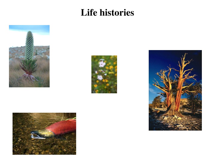
What is a life history? Life History An individual s pattern of allocation, throughout life, of time and energy to various fundamental activities, such as growth, reproduction, and repair of cell and tissue damage.
Examples of life history traits Size at birth Age specific reproductive investment Number, and size of offspring Age at maturity Length of life
Age specific reproductive investment x lx 1 mx 0 x lx 1 mx 0 1 1 2 .863 0 2 .863 .311 3 .778 0 3 .778 .412 4 .694 0 4 .694 .415 0.9 0.8 5 .610 0 5 .610 .512 0.7 6 .526 0 6 .526 .612 0.6 0.5 7 .442 .510 mx 7 .442 .611 0.4 8 .357 .612 8 .357 .656 0.3 9 .181 .712 0.2 9 .181 .557 0.1 10 .059 .713 10 .059 .442 0 0 5 10 15 11 .051 .745 11 .051 .358 Age, x 12 .042 .756 12 .042 .356 13 .034 .758 13 .034 .352 14 .025 .765 14 .025 .285 15 .017 .766 15 .017 .185 16 .009 .773 16 .009 .086
An extreme case: semalparity vs. iteroparity Semelparous Iteroparous x lx 1 mx 0 x lx 1 mx .125 1 1 2 .863 0 2 .863 .125 Semelparity A life history in which individuals reproduce only once in their lifetime. 3 .778 0 3 .778 .125 4 .694 0 4 .694 .125 5 .610 0 5 .610 .125 6 .526 0 6 .526 .125 Iteroparity A life history in which individuals reproduce more than once in their lifetime. 7 .442 0 7 .442 .125 8 .357 0 8 .357 .125 9 .181 0 9 .181 .125 10 .059 .125 10 .059 0 11 .051 .125 11 .051 0 12 .042 .125 12 .042 0 13 .034 .125 13 .034 0 14 .025 .125 14 .025 0 15 .017 .125 15 .017 0 16 .009 .125 16 .009 2.0
An example: Oncorhyncus mykiss Steelhead Rainbow trout Live a portion of their life in saltwater Spend entire life in freshwater Migrate to freshwater to spawn Iteroparous Often semelparous
An example: Mt Kenya Lobelias Lobelias live on Mt Kenya from 3300-5000m!
Mt Kenya Lobelias Lobelia telekii (semalparous) Lobelia keniensis (iteroparous)
Why be semalparous vs. iteroparous? A model of annuals vs. perennials: Cole (1954) = N B N + , 1 , A t A A t = + = ) 1 + ( N B N N B N + , 1 , , , P t P P t P t P P t B is the # of seeds produced (assumes that all seeds survive) Based on these equations, when would the relative numbers of annuals and perennials not change?
Coles Paradox The relative abundance of annuals and perennials will not change if their per capita growth rates are equal: = + 1 B B A P An annual need only produce one more seed per generation to out-reproduce a perennial. So why are there any perennials at all?
A resolution to Coles Paradox Assumptions of Cole s model No adult mortality in the perennial No juvenile mortality in either the annual or the perennial Relaxing these assumptions: Charnov and Schaffer (1973) Adults survive each year with probability Pa Juveniles survive to adulthood with probability Pj
A resolution to Coles Paradox = N P B N + , 1 , A t j A A t = + = + ( ) N P B N P N P B P N + , 1 , , , P t j P P t a P t j P a P t
A resolution to Coles Paradox The relative abundance of annuals and perennials will not change if their per capita growth rates are equal: = + P B P B P j A j P a Which after a little algebra is: P = + a B B A P P j Annuals (semalaparity) are favored by low adult survival and high juvenile survival Perennials (iteroparity) are favored by high adult survival and low juvenile survival
A resolution to Coles Paradox BP = 1, Pa = 1/2 BP = 1, Pj = 1/2 Annuals win Annuals win BA BA Perennials win Perennials win Juvenile survival, Pj Adult survival, Pa High rates of juvenile survival favor the evolution of annuals/semalparity High rates of adult survival favor the evolution of perennials/iteroparity
A test of the theory: Mt Kenya Lobelias Lobelia keniensis (iteroparous) Lobelia telekii (semalparous) 5000m (Dry rocky slopes) 3300m (Moist valley bottoms)
A test of the theory: Mt Kenya Lobelias Young (1990) Measured adult survival rates of the iteroparous species, Lobelia keniensis, at various sites along this environmental gradient Found that adult survival decreases as elevation increases and moisture decreases Found that the species transition zone occurs where adult survival falls below the critical threshold predicted by the model Adult mortality too high for iteroparity 5000m (Dry rocky slopes) Adult mortality sufficiently low for iteroparity 3300m (Moist valley bottoms)
-Practice question -In order to identify the importance of density regulation in a population of wild tigers, you assembled a data set drawn from a single population for which the population size and growth rate are known over a ten year period. This data is shown below. Does this data suggest population growth in this tiger population is density dependent? Why or why not? Year Population size Growth rate, r 1987 126 -0.11905 1988 111 -0.09009 1989 101 -0.11881 1990 89 -0.26966 1991 65 -0.29231 1992 46 -0.19565 1993 37 0.459459 1994 54 0.240741 1995 67 0.179104 1996 79 0.025316 1997 81 0.185185 1998 96 0.16 -What problems do you see with using this data to draw conclusions about density dependence?
Population size Year
Growth rate Population size
Number and size of offspring All else being equal it should be best to maximize the number of surviving offspring
A fundamental question Maternal resources Offspring Offspring
What is the best solution? The Lack Clutch The best solution is the one that maximizes the number of offspring surviving to maturity. Lack (1947) David Lack W = S*N
There is a fundamental trade-off W = N*S(N) 1 0.8 0.6 S 0.4 0.2 0 1 2 3 4 5 6 7 8 9 10 This is the Lack Clutch 4 3.5 3 2.5 W 2 1.5 1 0.5 0 1 2 3 4 5 6 7 8 9 10 Number of offspring produced, N
An example with #s N 2 4 6 8 10 S 1 W ? ? ? ? ? .75 .5 .25 .1 What is the optimal number of offspring to produce in this example?
An example with #s N 2 4 6 8 10 S 1 W 2 3 3 2 1 .75 .5 .25 .1 What is the optimal number of offspring to produce in this example?
Do real data conform to the Lack Clutch? The observed clutch sizes appear consistently smaller than the Lack Clutch Table from Stearns, 1992
Where does the Lack Clutch go wrong? Assumptions of the Lack Clutch 1. No trade-off between clutch size and maternal mortality 2. No trade-off between clutch size across years 3. No parent-offspring conflict (who controls clutch size anyway?) All have been shown to be important in some real cases!
For your current research position with the USFS, you have been tasked with developing a strategy for eliminating the invasive plant, Centaurea solstitialis. Because you have recognized that this plant appears to thrive when it is able to attract a large number of pollinators, you are hoping that you may be able to capitalize on Allee effects to drive invasive populations to extinction. Specifically, your idea is that if you can reduce the population size of this plant below some critical threshold with herbicide treatment, Allee effects will take over and lead to extinction. In order to evaluate the feasibility of your strategy, you have conducted controlled experiments where you estimate the growth rate, r, of experimental populations of this plant when grown at different densities. Your data is shown in the table below: Density (plants/m2) Growth rate (r) 35 30 25 20 15 10 5 A. Does your data suggest Allee effects operate in this system? Justify your response B. Additional studies conducted by others have demonstrated that herbicide application can reduce the population density of this plant, but never to densities below 17 plants/m2. Will your strategy for controlling this invasive plant work or not? Justify your response. 0.46 0.32 0.24 0.15 0.08 0.01 -0.05
Life history strategies: r vs. K selection In the 1960 s interest in life histories was stimulated by the identification of two broad classes of life history STRATEGIES (MacArthur and Wilson, 1967): r selected K selected Mature early Mature later Have many small offspring Have few large offspring Make a a few large reproductive efforts Make many small reproductive efforts Die young Live a long time
Putative examples of r vs. K selected species Taraxacum officinale Dandelion Sequoiadendron giganteum Redwood
Putative examples of r vs. K selected species Peromyscus leucopus Deer mouse Gopherus agassizii Desert tortoise
What conditions favor r vs K species? A simple model of density-dependent natural selection can help (Roughgarden, 1971) N = 1 [ ] N rN K of this, each INDIVIDUAL contributes: N = 1 [ r ] N K to population growth
A simple model of density dependent selection Since an individual s contribution to population growth is intimately connected to the notion of individual fitness, Roughgarden assumed the fitness of various genotypes is: N = + 1 1 ( ) W r AA AA K AA N = + 1 1 ( ) W r Aa Aa K Aa N = + 1 1 ( ) W r aa aa K aa Roughgarden (1971)
A critical assumption There is an inherent trade-off between K and r 12000 0.9 11000 0.8 10000 r 0.7 9000 K 0.6 8000 7000 0.5 AA Aa aa 1 2 3 Genotypes with a large r value tend to have a small K value
Can an allele that increases r but decreases K fix? 1 1000 N Example 1: rAA = .15 KAA = 900 rAa = .10 KAa = 950 raa = .05 Kaa = 1000 0.8 800 0.6 600 p N 0.4 400 p 0.2 200 0 0 0 200 400 600 800 1000 1 1000 N 0.8 800 Example 2: rAA = .30 KAA = 950 rAa = .20 KAa = 975 raa = .10 Kaa = 1000 0.6 600 p N 0.4 400 p 0.2 200 0 0 0 200 400 600 800 1000 Generation # In a constant environment, NO!
Why does the r selected genotype lose? In a constant environment the population will ultimately approach its carrying capacity As the population size approaches the carrying capacity of the various genotypes, density dependent selection becomes strong Under these conditions, genotypes with a high K are favored by natural selection
What about disturbed environments? 1 1000 0.8 N 800 In the examples at right, the population size is reduced (disturbed) by a random amount in each generation. 0.6 600 p N 0.4 400 p 0.2 200 0 0 Disturbance increases 0 200 400 600 800 1000 In this example: rAA = .30 KAA = 900 rAa = .20 KAa = 950 raa = .10 Kaa = 1000 1 1000 0.8 800 N p 0.6 600 p N 0.4 400 0.2 200 0 0 0 200 400 600 800 1000 1 1000 p 0.8 800 0.6 600 N p N 0.4 400 0.2 200 0 0 0 200 400 600 800 1000 Generation #
Conclusions for rand K selection In a constant environment the population will ultimately approach its carrying capacity and the genotype with the highest K will become fixed If population size remains sufficiently below the K s of the various genotypes due to random environmental disturbances or other factors, the genotype with the highest r will become fixed in the population
A test of rvs. K selection: Dandelions and disturbance (Solbrig, 1971) Four genotypes A-D. - Genotype A has the largest allocation to rapid seed production - Genotype D delays reproduction until after substantial leaf formation - Genotypes B and C are intermediate Established three plots with varying levels of disturbance - Heavily disturbed by weekly lawn mowing - Moderately disturbed with monthly lawn mowing - Minimal disturbance with seasonal lawn mowing
Dandelions and disturbance (Solbrig, 1971) rselected genotype Kselected genotype Disturbance level A B C D Early Late Reproduction 73 53 17 Reproduction 0 1 64 High Medium Low 13 32 8 14 14 11 - High levels of disturbance favored the genotype with the greatest r


")