Linear Algebra Applications in Engineering and Data Analysis
Explore the applications of linear algebra in various fields such as engineering, network analysis, population growth, optimization, signal processing, statistics, computer graphics, and more. Learn how matrices and vectors play a crucial role in solving real-world problems efficiently.

Download Presentation

Please find below an Image/Link to download the presentation.
The content on the website is provided AS IS for your information and personal use only. It may not be sold, licensed, or shared on other websites without obtaining consent from the author. If you encounter any issues during the download, it is possible that the publisher has removed the file from their server.
You are allowed to download the files provided on this website for personal or commercial use, subject to the condition that they are used lawfully. All files are the property of their respective owners.
The content on the website is provided AS IS for your information and personal use only. It may not be sold, licensed, or shared on other websites without obtaining consent from the author.
E N D
Presentation Transcript
Numpy Charlie Dey Director, Training and Professional Development charlie@tacc.utexas.edu
Monte Carlo Pi
Sequential Algorithm A Monte Carlo algorithm for approximating uniformly generates the points in the square [-1, 1] x [-1, 1]. Then it counts the points which lie in the inside of the unit circle.
Sequential Algorithm A Monte Carlo algorithm for approximating uniformly generates the points in the square [-1, 1] x [-1, 1]. Then it counts the points which lie in the inside of the unit circle.
Sequential Algorithm An approximation of is then computed by the following formula:
Algorithm double approximatePi(int numSamples) { float x, y; int counter = 0; for (int s = 0; s != numSamples; s++) { x = random number between -1, 1; y = random number between -1, 1; if (x * x + y * y < 1) { counter++; } } return 4.0 * counter / numSamples; } Let's code this in Python, Google to see what command in Python produces a random number
Linear Algebra Applications Matrices in Engineering, such as a line of springs. Graphs and Networks, such as analyzing networks. Markov Matrices, Population, and Economics, such as population growth. Linear Programming, the simplex optimization method. Fourier Series: Linear Algebra for functions, used widely in signal processing. Linear Algebra for statistics and probability, such as least squares for regression. Computer Graphics, such as the various translation, rescaling and rotation of images. 7
Linear Algebra Linear algebra is about linear combinations. Using math on columns of numbers called vectors and arrays of numbers called matrices to create new columns and arrays of numbers. Linear algebra is the study of lines and planes, vector spaces and mappings that are required for linear transforms. 8
Linear Algebra Linear algebra is the mathematics of data. Matrices and vectors are the language of data. Let's look at the following: y = 4 * x + 1 describes a line on a two-dimensional graph 9
Linear Algebra Linear algebra is the mathematics of data. Matrices and vectors are the language of data. Let's look at the following: y = 0.1 * x1 + 0.4 * x2 y = 0.3 * x1 + 0.9 * x2 line up a system of equations with the same form with two or more unknowns 10
Linear Algebra Linear algebra is the mathematics of data. Matrices and vectors are the language of data. Let's look at the following: 1 = 0.1 * x1 + 0.4 * x2 3 = 0.3 * x1 + 0.9 * x2 line up a system of equations with the same form with two or more unknowns 11
Linear Algebra Linear algebra is the mathematics of data. Matrices and vectors are the language of data. Let's look at the following, Ax = b : 5 = 0.1 * x1 + 0.4 * x2 + x3 10 = 0.3 * x1 + 0.9 * x2 + 2.0 * x3 3 = 0.2 * x1 + 0.3 * x2 - .5 * x3 ls there a x1, x2, x3 that solves this system? 12
Linear Algebra Gaussian Elimination The goals of Gaussian elimination are to make the upper-left corner element a 1 use elementary row operations to get 0s in all positions underneath that first 1 get 1s for leading coefficients in every row diagonally from the upper-left to lower-right corner, and get 0s beneath all leading coefficients. you eliminate all variables in the last row except for one, all variables except for two in the equation above that one, and so on and so forth to the top equation, which has all the variables. Then use back substitution to solve for one variable at a time by plugging the values you know into the equations from the bottom up.. 13
Linear Algebra Gaussian Elimination, Rules You can multiply any row by a constant (other than zero). You can switch any two rows. You can add two rows together. 14
Linear Algebra Transpose A defined matrix can be transposed, which creates a new matrix with the number of columns and rows flipped. This is denoted by the superscript T next to the matrix. An invisible diagonal line can be drawn through the matrix from top left to bottom right on which the matrix can be flipped to give the transpose. 15
Linear Algebra Inversion Matrix inversion is a process that finds another matrix that when multiplied with the matrix, results in an identity matrix. Given a matrix A, find matrix B, such that AB or BA = In. The operation of inverting a matrix is indicated by a -1 superscript next to the matrix; for example, A^-1. The result of the operation is referred to as the inverse of the original matrix; for example, B is the inverse of A. 16
Linear Algebra Trace A trace of a square matrix is the sum of the values on the main diagonal of the matrix (top-left to bottom-right). 17
Linear Algebra Determinant The determinant of a square matrix is a scalar representation of the volume of the matrix. The determinant describes the relative geometry of the vectors that make up the rows of the matrix. More specifically, the determinant of a matrix A tells you the volume of a box with sides given by rows of A. Page 119, No Bullshit Guide To Linear Algebra, 2017 18
Linear Algebra Matrix Rank The rank of a matrix is the estimate of the number of linearly independent rows or columns in a matrix. 19
Linear Algebra - Matrix Arithmetic Matrix Addition Two matrices with the same dimensions can be added together to create a new third matrix. C = A + BC[0,0] = A[0,0] + B[0,0] C[1,0] = A[1,0] + B[1,0] C[2,0] = A[2,0] + B[2,0] C[0,1] = A[0,1] + B[0,1] C[1,1] = A[1,1] + B[1,1] C[2,1] = A[2,1] + B[2,1] 20
Linear Algebra - Matrix Arithmetic Matrix Subtraction Similarly, one matrix can be subtracted from another matrix with the same dimensions. C = A - B C[0,0] = A[0,0] - B[0,0] C[1,0] = A[1,0] - B[1,0] C[2,0] = A[2,0] - B[2,0] C[0,1] = A[0,1] - B[0,1] C[1,1] = A[1,1] - B[1,1] C[2,1] = A[2,1] - B[2,1] 21
Linear Algebra - Matrix Arithmetic Matrix Multiplication (Hadamard Product) Two matrices with the same size can be multiplied together, and this is often called element- wise matrix multiplication or the Hadamard product. It is not the typical operation meant when referring to matrix multiplication, therefore a different operator is often used, such as a circle o . C = A o B C[0,0] = A[0,0] * B[0,0] C[1,0] = A[1,0] * B[1,0] C[2,0] = A[2,0] * B[2,0] C[0,1] = A[0,1] * B[0,1] C[1,1] = A[1,1] * B[1,1] C[2,1] = A[2,1] * B[2,1] 22
Linear Algebra - Matrix Arithmetic Matrix Division One matrix can be divided by another matrix with the same dimensions. C = A / B C[0,0] = A[0,0] / B[0,0] C[1,0] = A[1,0] / B[1,0] C[2,0] = A[2,0] / B[2,0] C[0,1] = A[0,1] / B[0,1] C[1,1] = A[1,1] / B[1,1] C[2,1] = A[2,1] / B[2,1] 23
Linear Algebra - Matrix Arithmetic Matrix-Matrix Multiplication (Dot Product) Matrix multiplication, also called the matrix dot product is more complicated than the previous operations and involves a rule as not all matrices can be multiplied together. One of the most important operations involving matrices is multiplication of two matrices. The matrix product of matrices A and B is a third matrix C. In order for this product to be defined, A must have the same number of columns as B has rows. If A is of shape m n and B is of shape n p, then C is of shape m p. Page 34, Deep Learning, 2016. 24
Linear Algebra - Matrix Arithmetic Matrix-Matrix Multiplication (Dot Product) a11, a12 a21, a22 a31, a32 A = b11, b12 B = b21, b22 a11 * b11 + a12 * b21, a11 * b12 + a12 * b22 C = a21 * b11 + a22 * b21, a21 * b12 + a22 * b22 a31 * b11 + a32 * b21, a31 * b12 + a32 * b22 25
Numerical Linear Algebra, Two Different Approaches Solve Ax = b Direct methods: Deterministic Exact up to machine precision Expensive (in time and space) Iterative methods: Only approximate Cheaper in space and (possibly) time Convergence not guaranteed
Iterative Methods Choose any x0and repeat until or until
Example of Iterative Solution Example system with solution (2,1,1) Suppose you know (physics) that solution components are roughly the same size, and observe the dominant size of the diagonal, then might be a good approximation: solution (2.1, 9/7, 8/6)
Iterative Example Example system with solution (2,1,1) Also easy to solve: with solution (2.1, 7.95/7, 5.9/6)
Iterative Example Instead of solving we solved Look for the missing part: , then Solve again and update . Two decimals per iteration. This is not typical Exact system solving: O(n3) cost; iteration: O(n2) per iteration. Potentially cheaper
Abstract Presentation To solve Ax = b; too expensive; suppose K A and solving Kx = b is possible Define Kx0= b, then error correction x0= x + e0, and A(x0- e0) = b so Ae0= Ax0- b = r0; this is again unsolvable, so K 0and x1= x0- 0 Now iterate: e1= x1- x, Ae1= Ax1- b = r1et cetera
Error Analysis One step Inductively: Geometric reduction (or amplification!) This is 'stationary iteration': every iteration step the same. Simple analysis, limited applicability
Computationally If A = K -N then Ax = b Kx = Nx + b Kxi+1= Nxi+ b (because Kx = Nx +b is a "fixed point" of an iteration) Equivalent to the above, and you don't actually need to form the residual
Choice of K The closer K is to A, the faster the convergence Diagonal and lower triangular choice mentioned above: let A = DA+ LA+ UA be a splitting into diagonal, lower triangular, upper triangular part, then Jacobi method: K = DA(diagonal part), Gauss-Seidel method: K = DA+ LA(lower triangle, including diagonal) SOR method:
Jacobi Method Given a square system of n linear equations: where:
Jacobi Method Then A can be decomposed into a diagonal component D, and the remainder R:
Jacobi Method The solution is then obtained iteratively via The computation of xi(k+1)requires each element in x(k)except itself. Unlike the Gauss Seidel method, we can't overwrite xi(k)with xi(k+1), as that value will be needed by the rest of the computation. The minimum amount of storage is two vectors of size n.
Jacobi Method Algorithm. Choose your initial guess, x[0] Start iterating, k=0 While not converged do Start your i-loop (for i = 1 to n) sigma = 0 Start your j-loop (for j = 1 to n) If j not equal to i sigma = sigma + a[i][j] * x[j]k End j-loop x[i]k= (b[i] sigma)/a[i][i] End i-loop Check for convergence Iterate k, ie. k = k+1
What about the Lower and Upper Triangles? If we write D, L, and U for the diagonal, strict lower triangular and strict upper triangular and parts of A, respectively, then Jacobi s Method can be written in matrix-vector notation as so that
Gauss-Seidel K = DA + LA Algorithm: for k = 1, ... until convergence, do: for i = 1 ... n: Ax=b => (DA+LA+UA)x=b (DA+LA)xk+1= -UAxk+ b {DA}ii=aii{UA or LA}ij=aiji j Implementation: for k = 1, ... until convergence, do: for i = 1 ... n:
Gauss-Seidel Method Given a square system of n linear equations: where:
Gauss-Seidel Method The system of linear equations may be rewritten as:
Gauss-Seidel Method Which gives us:
Gauss-Seidel Method Algorithm: Choose your initial guess, theta[0] While not converged do: Start your i-loop (for i = 1 to n) sigma = 0 Start your j-loop (for j = 1 to n) If j not equal to i End j-loop theta[i] = (b[i] sigma)/a[i][i] End i-loop Check for convergence iterate sigma = sigma + a[i][j] * theta[j]
Stopping Tests When to stop converging? Can size of the error be guaranteed? Direct tests on error en= x - xnimpossible; two choices Relative change in the computed solution small: Residual small enough: Without proof: both imply that the error is less than some other
Python Python - - NumPy "Numerical Python" open source extension module for Python provides fast precompiled functions for mathematical and numerical routines adds powerful data structures for efficient computation of multi-dimensional arrays and matrices. 48
NumPy, First Steps , First Steps Let build a simple list, turn it into a numpy array and perform some simple math. import numpy as np cvalues = [25.3, 24.8, 26.9, 23.9] C = np.array(cvalues) print(C) 49
NumPy, First Steps , First Steps Let build a simple list, turn it into a numpy array and perform some simple math. print(C * 9 / 5 + 32) vs. fvalues = [ x*9/5 + 32 for x in cvalues] print(fvalues) 50