Linear Programming Techniques: Simplex Method and Duality Explained
Learn how to apply the Simplex method and duality in Linear Programming to showcase near-optimality of solutions. Discover the mechanics of deriving a dual LP and understand how to utilize duality effectively. Explore a step-by-step example solving a generic LP using the Simplex algorithm.
Download Presentation

Please find below an Image/Link to download the presentation.
The content on the website is provided AS IS for your information and personal use only. It may not be sold, licensed, or shared on other websites without obtaining consent from the author. If you encounter any issues during the download, it is possible that the publisher has removed the file from their server.
You are allowed to download the files provided on this website for personal or commercial use, subject to the condition that they are used lawfully. All files are the property of their respective owners.
The content on the website is provided AS IS for your information and personal use only. It may not be sold, licensed, or shared on other websites without obtaining consent from the author.
E N D
Presentation Transcript
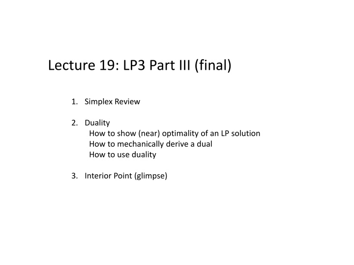
Lecture 19: LP3 Part III (final) 1. Simplex Review 2. Duality How to show (near) optimality of an LP solution How to mechanically derive a dual How to use duality 3. Interior Point (glimpse)
Simplex (example) example from Understanding and Using Linear Programming by Jiri Matousek and Bernd Gaertner.
Show how to solve a generic LP of the form max ??? ?? ? ? 0 Algorithm by example: 2 vars.
?2 ?1 Replace all the inequality constraints by equalities, using slack variables ?1 + ?2 1 ?1 + ?2 + ?3= 1 and ?3 0
Replace all the inequality constraints by equalities, using slack variables All examples on the following slides have form: max c.x s.t. Ax = b x 0 won t explicitly write, but always there!
Now: stop writing the non-negativity constraints rewrite each equality to move ?1, ?2 on the right hand side. ?1+ ?2+ ?3= 1 ?3= 1 + ?1 ?2 let ? denote objective value
Invariant: 2 vars on the right (in general: #(original vars) vars on RHS) they have values zero write other vars, and objective, in terms of these RHS vars. LHS values are fully determined by RHS (due to equalities).
Setting ?1,?2 to zero gives solution: (x1 = 0, x2 = 0, x3 = 1, x4 = 3, x5 = 2) Invariant: 2 vars on the right (in general: #(original vars) vars on RHS) they have values zero write other vars, and objective, in terms of these RHS vars. LHS values are fully determined by RHS (due to equalities).
Setting ?1,?2 to zero gives solution: (x1 = 0, x2 = 0, x3 = 1, x4 = 3, x5 = 2) Objective z is ?1+ ?2= 0 + 0 = 0. How can we increase it? Maybe raise one of the vars ?1 or ?2?
(x1 = 0, x2 = 0, x3 = 1, x4 = 3, x5 = 2) Pick a RHS variable (say x2) with positive coefficient in objective Increase its value. This increases the objective z. How far can we increase ?2? Can increase until some other variable (x3) goes to 0. Then stop. Note: red inequality that became tight corresponds to red constraint that we hit in the picture. Not a coincidence, actually.
(x1 = 0, x2 = 1, x3 = 0, x4 = 3, x5 = 1) OK: progress! Objective is now 1. But we don t have the structure we wanted: Invariant: 2 vars on the right (in general: equals number of original vars) they have values zero not true all other vars, and the objective, in terms of RHS vars. So fix it: we just made ?3 zero. Move it to RHS, move ?2 to LHS, and rewrite!
(x1 = 0, x2 = 1, x3 = 0, x4 = 3, x5 = 1) (Make sure you re happy with how we rewrote the LP.) e.g., used to be ?5= 2 ?2, so substituting in ?2= 1 + ?1 ?3 we get ?5= 2 1 + ?1 ?3 = 1 ?1+ ?3
(x1 = 0, x2 = 1, x3 = 0, x4 = 3, x5 = 1) And continue. To increase objective find var ?? with positive coefficient in objective raise it until some other var ?? on left becomes zero. move ?? to right, ?? to left write all other constraints in terms of (new) set of RHS vars Repeat.
(x1 = 0, x2 = 1, x3 = 0, x4 = 3, x5 = 1) Let s run this process: Pick a RHS variable (say x1) with positive coefficient in objective Increase its value until some other variable (x5) goes to 0 x1 goes to LHS, x5 goes to RHS.
(x1 = 1, x2 = 2, x3 = 0, x4 = 2, x5 = 0) Pick a RHS variable (say x3) with positive coefficient in objective Increase its value until some other variable (x4) goes to 0 x3 goes to LHS, x4 goes to RHS.
(x1 = 3, x2 = 2, x3 = 2, x4 = 0, x5 = 0) Pick a RHS variable with positive coefficient in objective if no such variable, must be at optimum. Why can t it be higher? z is just restatement of original objective function (just used equalities) Any other (non-negative) setting of RHS variables gives worse value.
Unboundedness Pick a RHS variable (say x2) with positive coefficient in objective If it can be increased arbitrarily, LP value is unbounded
Degeneracy Pick a RHS variable (say x2) with positive coefficient in objective raise it. but since ?1= 0, can only increase ?2 by zero too. If it can be increased by only zero, degenerate vertex. But still move ?2 to LHS, ?3 to RHS
Degeneracy Pick a RHS variable (say x1) with positive coefficient in objective now it can be increased What if we keep cycling at degenerate vertices (or degenerate faces)? Solution: anti-cycling pivot rules.
Pivot rules If choice of many variables to raise, which one to raise? called a pivot rule . Here are some examples: largest coefficient largest increase steepest edge often best in practice Bland s rule (non-cycling) Random edge Good rule can find short paths to an optimal vertex Also, prevent cycling at degenerate vertices

