Linear Regression and Correlation in Data Analysis
Linear regression and correlation analysis in statistics involve examining the relationship between explanatory and response variables to determine if there is a linear association. By estimating parameters like intercept and slope, the model seeks to minimize errors and predict outcomes accurately. An example scenario involving pharmacodynamics of LSD response showcases how this method can be applied in real-world data analysis.

Download Presentation

Please find below an Image/Link to download the presentation.
The content on the website is provided AS IS for your information and personal use only. It may not be sold, licensed, or shared on other websites without obtaining consent from the author.If you encounter any issues during the download, it is possible that the publisher has removed the file from their server.
You are allowed to download the files provided on this website for personal or commercial use, subject to the condition that they are used lawfully. All files are the property of their respective owners.
The content on the website is provided AS IS for your information and personal use only. It may not be sold, licensed, or shared on other websites without obtaining consent from the author.
E N D
Presentation Transcript
Section 9.1 Linear Regression and Correlation
Linear Regression and Correlation Explanatory and Response Variables are Numeric Relationship between the mean of the response variable and the level of the explanatory variable assumed to be approximately linear (straight line) Model: ( ) = + + ~ 0, Y X N 0 1 1 > 0 Positive Association 1 < 0 Negative Association 1 = 0 No Association
Least Squares Estimation of 0, 1 0 Mean response when x=0 (y-intercept) 1 Change in mean response when X increases by 1 unit (slope) 0, 1 are unknown parameters (like ) 0+ 1X Mean response when explanatory variable takes on the value X Goal: Choose values (estimates) that minimize the sum of squared errors (SSE) of observed values to the straight-line: 2 2 ^ ^ ^ ^ ^ ^ n n = + = = + Y X SSE Y Y Y X i 0 1 0 1 i i i = = 1 1 i i
Least Squares Computations Parameter Estimates Summary Calculations ( )( ) ( ( ( ) )( 2 X X Y Y = S X X S S ^ = = XX XY ( ) 1 ) 2 X X = S X X Y Y XX XY ) ^ ^ 2 = = S Y Y Y X YY 0 1 2 ^ = SSE Y Y 2 n ^ Y Y ( ) i i SSE n = 2 XY S S S = = = 2 = 1 i s MSE YY XX 2 2 n
Example - Pharmacodynamics of LSD Response (Y) - Math score (mean among 5 volunteers) Predictor (X) - LSD tissue concentration (mean of 5 volunteers) Score (y) 78.93 58.20 67.47 37.47 45.65 32.92 29.97 LSD Conc (x) 1.17 2.97 3.26 4.69 5.83 6.00 6.41 Source: Wagner, Agahajanian, and Bing (1968). Correlation of Performance Test Scores with Tissue Concentration of Lysergic Acid Diethylamide in Human Subjects. Clinical Pharmacology and Therapeutics, Vol.9 pp635-638.
Example - Pharmacodynamics of LSD Score (y) 78.93 58.20 67.47 37.47 45.65 32.92 29.97 350.61 LSD Conc (x) 1.17 2.97 3.26 4.69 5.83 6.00 6.41 30.33 x-xbar -3.163 -1.363 -1.073 0.357 1.497 1.667 2.077 -0.001 y-ybar 28.843 8.113 17.383 -12.617 -4.437 -17.167 -20.117 0.001 Sxx Sxy Syy 10.004569 1.857769 1.151329 0.127449 2.241009 2.778889 4.313929 22.474943 -91.230409 -11.058019 -18.651959 -4.504269 -6.642189 -28.617389 -41.783009 -202.487243 2078.183343 831.918649 65.820769 302.168689 159.188689 19.686969 294.705889 404.693689 (Column totals given in bottom row of table) 350.61 7 202.4872 22.4749 30.33 7 = = = = 50.087 4.333 Y X ^ ^ ^ = = = = 50.09 ( 9.01)(4.33) = 9.01 89.10 Y X 1 0 1 ^ = 89.10 9.01 = = = = = 2 50.72 50.72 7.12 Y X s MSE s MSE
Example Berry Chewiness and Sugar Content Response Variable (Y) Berry Chewiness (mJ) Predictor Variable (X) Sugar Content (grams/liter) Sugar levels: 176.5 192.6 209.3 225.0 242.1 258.5 ni = 15 replicates per sugar level: n = 6(15) = 90 X Y01 Y02 Y03 Y04 Y05 Y06 Y07 176.5 2.1381 3.6588 4.7656 1.1835 3.7518 1.8404 2.2266 192.6 2.2918 3.9924 3.0021 3.4332 3.6314 1.6526 3.7707 209.3 2.7466 1.8552 2.6526 3.1171 2.5941 3.4251 3.9640 225.0 1.6433 2.0722 2.1001 4.3682 2.3977 0.9950 4.4895 242.1 2.2401 2.0816 1.4054 1.1273 2.0976 1.4141 2.1817 258.5 1.2349 1.6900 1.9316 2.6551 1.9119 2.1120 2.3469 Y08 4.1262 3.3163 3.3389 0.8833 2.2254 2.0400 Y09 4.9845 3.6039 0.6925 2.6824 3.2145 1.5142 Y10 5.5386 4.4036 3.3025 3.4452 3.3571 1.5389 Y11 4.3668 3.4560 2.7557 3.7186 1.2011 1.7064 Y12 4.4714 3.7380 3.9685 3.1528 1.2226 1.2969 Y13 2.4990 4.2960 3.2016 1.3621 2.3168 1.0169 Y14 2.8283 3.0917 3.9999 3.1512 1.4921 0.4185 Y15 3.0703 3.4703 3.0857 4.1883 2.5725 2.2360 = = 217.3333 70657.4 = 2.7083 = X S Y S = 1610.776 110.8472 S XX XY YY 74.126 90 2 ^ = 7.6629 0.0228 = = = 2 Fitted Equation: 74.126 0.842 Y X SSE s Source: I. Zouid, R. Siret, F. Jourjion, E. Mehinagic, L. Rolle (2013)."Impact of Grapes Heterogeneity According to Sugar Level on Both Physical and Mechanical Berries Properties and their AnthocyaninsExtractability at Harvest," Journal of Texture Studies, Vol. 44, pp. 95-103.
74.126 90 2 ^ = 7.6629 0.0228 = = = 2 Fitted Equation: 74.126 0.842 Y X SSE s
Inference Concerning the Slope (1) Parameter: Slope in the population model( 1) Estimator: Least squares estimate: Estimated standard error: ^ 1 MSE ^ ^ = SE 1 ( ) n 2 X X i = 1 i Methods of making inference regarding population: Hypothesis tests (2-sided or 1-sided) Confidence Intervals
Hypothesis Test for 1 1-sided Test H0: 1 = 0 HA+: 1 > 0 or HA-: 1 < 0 2-Sided Test H0: 1 = 0 HA: 1 0 ^ ^ = . .: T S t 1 = . .: T S t 1 obs MSE S t obs MSE S XX XX . .:| R R | t + . . : R R . . : R R t t t t /2, 2 t obs n , 2 , 2 obs n obs n + P val P val value:2 ( | |) : ( P t ) : ( P t ) P P t t t obs obs obs
(1-)100% Confidence Interval for 1 MSE S ^ ^ ^ ^ t SE t 1 1 1 /2 /2, 2 n XX Conclude positive association if entire interval above 0 Conclude negative association if entire interval below 0 Cannot conclude an association if interval contains 0 Conclusion based on interval is same as 2-sided hypothesis test
Example - Pharmacodynamics of LSD ^ = = = = = 2 7 9.01 50.72 22.475 n s MSE S 1 XX 50.72 22.475 ^ ^ = = 1.50 SE 1 Testing H0: 1 = 0 vs HA: 1 0 9.01 1.50 = = = . .: T S t 6.01 . .:| R R | 2.571 t .025,5 t obs obs 95% Confidence Interval for 1 : . 9 . 9 . 5 01 . 2 571 . 1 ( 50 ) 01 . 3 86 ( 12 87 . , 15 )
R Output Estimates, t-tests, CIs mathlsd.reg <- lm(math ~ lsd) summary(mathlsd.reg) confint(mathlsd.reg) > summary(mathlsd.reg) Coefficients: Estimate Std. Error t value Pr(>|t|) (Intercept) 89.124 7.048 12.646 5.49e-05 *** lsd -9.009 1.503 -5.994 0.00185 ** Residual standard error: 7.126 on 5 degrees of freedom Residual standard error: 7.126 on 5 degrees of freedom Multiple R-squared: 0.8778, Adjusted R-squared: 0.8534 F-statistic: 35.93 on 1 and 5 DF, p-value: 0.001854 > confint(mathlsd.reg) 2.5 % 97.5 % (Intercept) 71.00758 107.240169 lsd -12.87325 -5.145685
Plot of Data and Equation mathlsd.reg <- lm(math ~ lsd) plot(math~lsd, main= X=LSD Concentration, Y=Mean Math Score ) abline(mathlsd.reg)
Example Berry Chewiness and Sugar Content ^ = 0.0228 = = = = 2 90 0.842 70657.4 n s MSE S 1 XX 0.842 70657.4 ^ ^ = = 0.00345 SE 1 Testing H0: 1 = 0 vs HA: 1 0 0.0228 0.00345 = = = . .: T S t 6.603 . .:| R R | 1.987 t .025,88 t obs obs 95% Confidence Interval for 1 : 0.0228 1.987(0.00345) 0.0228 0.0069 ( 0.0297, 0.0159)
Confidence Interval for Mean When X=X* Mean Response at a specific level X* is = = = + * * * ( | ) E Y X X X 0 1 Estimated Mean response and standard error (replacing unknown 0 and 1 with estimates): ( ) 2 * X X * * 1 n ^ ^ ^ ^ ^ = + = + * Y X SE Y MSE 0 1 S XX Confidence Interval for Mean Response: ( ) 2 * X X * * * 1 n ^ ^ ^ ^ + Y t SE Y Y t MSE /2, 2 /2, 2 n n S XX
Prediction Interval of Future Response @ X=X* Response at a specific level X* is = + = + + * * * New Y X 0 1 Estimated response and standard error (replacing unknown 0 and 1 with estimates): ( ) 2 * X X * * 1 n ^ ^ ^ ^ ^ = + = + + * 1 Y X SE Y MSE New New 0 1 S XX Prediction Interval for Future Response: ( ) 2 * X X * * * 1 n ^ ^ ^ ^ + + 1 Y t SE Y Y t MSE New New New /2, 2 /2, 2 n n S XX
Example 95% CI and PI when Sugar = 215.0 R command give the 95% CI s and PI s when X* = 215 for berries berry.mod1 <- lm(chewiness ~ sugar) Xstar <- 215 predict(berry.mod1, list(sugar=Xstar), int="confidence") predict(berry.mod1, list(sugar=Xstar), int="prediction") > predict(berry.mod1, list(sugar=Xstar), int="confidence") fit lwr upr 1 2.761525 2.568601 2.954449 > predict(berry.mod1, list(sugar=Xstar), int="prediction") fit lwr upr 1 2.761525 0.9274281 4.595622
Correlation Coefficient Measures the strength of the linear association between two variables Takes on the same sign as the slope estimate from the linear regression Not effected by linear transformations of Y or X Does not distinguish between dependent and independent variable (e.g. height and weight) Population Parameter: YX Pearson s Correlation Coefficient: S = 1 1 YX r YX r XY S S XX YY
Correlation Coefficient Values close to 1 in absolute value strong linear association, positive or negative from sign Values close to 0 imply little or no association If data contain outliers (are non-normal), Spearman s coefficient of correlation can be computed based on the ranks of the X and Y values Test of H0: YX = 0 is equivalent to test of H0: 1=0 Coefficient of Determination (rYX2) - Proportion of variation in Y explained by the regression on X: (Total) (Residual) (Total) S SSE SS SS = = = 2 2 2 ( ) 0 1 YX r YX r YX r YY S SS YY
Example - Pharmacodynamics of LSD = 202.487 = = = 22.475 2078.183 253.89 S S S SSE XX XY YY 202.487 = = 0.9369 YX r (22.475)(2078.183) 2078.183 2078.183 253.89 = = ( 0.9369) = 2 2 0.8778 YX r
Example EXCEL and R Output Pearson s and Spearman s Measures obs lsd (X) math (Y) rank(X) 78.93 58.2 67.47 37.47 45.65 32.92 29.97 rank(Y) r(X)-4 r(Y)-4 (r(X)-4)(r(Y)-4) 1 2 3 4 5 6 7 1.17 2.97 3.26 4.69 5.83 1 2 3 4 5 6 7 7 5 6 3 4 2 1 -3 -2 -1 0 1 2 3 0 28 3 1 2 -9 -2 -2 0 0 -4 -9 -1 0 -2 -3 0 28 Spearman's Rho 6 6.41 Sum SumSq -26 -0.9286 > cor(math, lsd) [1] -0.9369285 > cor(math, lsd, method="spearman") [1] -0.9285714
Hypothesis Test for YX 1-sided Test H0: YX = 0 HA+: YX > 0 or HA-: YX < 0 2-Sided Test H0: YX = 0 HA: YX 0 2 n = . .: T S t YX r 2 n = . .: T S t YX r obs 2 1 YX r obs 2 1 YX r . .:| R R | t t + . . : R R . . : R R t t t t /2, 2 t obs n , 2 , 2 obs n obs n + P val P val value:2 ( | |) P P t : ( P t ) : ( P t ) t t obs obs obs
R Commands and Output LSD Data math <- c(78.93,58.20,67.47,37.47,45.65,32.92,29.97) lsd <- c(1.17,2.97,3.26,4.69,5.83,6.00,6.41) cor.test(math,lsd) cor.test(math,lsd) Pearson's product-moment correlation data: math and lsd t = -5.994, df = 5, p-value = 0.001854 alternative hypothesis: true correlation is not equal to 0 95 percent confidence interval: -0.9908681 -0.6244782 sample estimates: cor -0.9369285
R Commands and Output Berry Data ## Pearson product moment coefficient of correlation and test of H0: rho=0 cor(chewiness, sugar) cor.test(chewiness, sugar) > cor(chewiness, sugar) [1] -0.5755643 > cor.test(chewiness, sugar) Pearson's product-moment correlation data: chewiness and sugar t = -6.6025, df = 88, p-value = 2.951e-09 alternative hypothesis: true correlation is not equal to 0 95 percent confidence interval: -0.6993026 -0.4183365 sample estimates: cor -0.5755643
Analysis of Variance in Regression Goal: Partition the total variation in Y into random variation and variation explained by X ) i Y Y Y Y Y = + = = ( ^ ^ Y i i i 2 2 ( ) n n n ^ ^ 2 + = + TSS Y Y Y Y Y Y SSE SSR i i i i = = = 1 1 1 i i i These three sums of squares and degrees of freedom are: Total (TSS) DFT = n-1 Error (SSE) DFE = n-2 Model (SSR) DFR = 1
Analysis of Variance for Regression Source of Variation Model Error Total Sum of Squares SSR SSE TSS Degrees of Freedom 1 n-2 n-1 Mean Square MSR = SSR/1 MSE = SSE/(n-2) F F = MSR/MSE Analysis of Variance - F-test H0: 1 = 0 HA: 1 0 MSR = . : . S T F obs MSE . : . R R F F , 1 , F 2 F obs n value : ( ) P P obs
Example - Pharmacodynamics of LSD Total Sum of squares: ( ) n 2 = = 7 1 = = 2078.183 6 TSS Y Y DF i T = 1 i Error Sum of squares: 2 n ^ = = 7 2 = = 253.890 5 SSE Y Y DF i i E = 1 i Model Sum of Squares: 2 n ^ = = 2078.183 253.890 1824.293 = = 1 SSR Y Y DF i R = 1 i
Example - Pharmacodynamics of LSD Source of Variation Model Error Total Sum of Squares 1824.293 253.890 2078.183 Degrees of Freedom 1 5 6 Mean Square 1824.293 50.778 F 35.93 Analysis of Variance - F-test H0: 1 = 0 HA: 1 0 MSR MSE = = . .: T S F 35.93 obs = . .: R R F 6.61 .05,1,5 F P F obs 35.93) .0019 = -value: ( P 1,5
Example - R Output LSD Data mathlsd.reg <- lm(math ~ lsd) anova(mathlsd.reg) > anova(mathlsd.reg) Analysis of Variance Table Response: math Df Sum Sq Mean Sq F value Pr(>F) lsd 1 1824.30 1824.30 35.928 0.001854 ** Residuals 5 253.88 50.78
Example - R Output Berry Data ## Analysis of Variance and F-test berry.mod1 <- lm(chewiness ~ sugar) anova(berry.mod1) > berry.mod1 <- lm(chewiness ~ sugar) > anova(berry.mod1) Analysis of Variance Table Response: chewiness Df Sum Sq Mean Sq F value Pr(>F) sugar 1 36.721 36.721 43.594 2.951e-09 *** Residuals 88 74.126 0.842
Linearity of Regression (SLR) -Test for Lack-of-Fit ( observations at distinct levels of " ") c F n X j ( ) ( ) = + = + : : H E Y X H E Y X 0 0 1 0 1 i i A i i i Compute fitted value and sample mean for each distinct level Y Y X j j ( ) n c j 2 ( ) = = Lack-of-Fit: 2 SS LF Y Y df c j j LF = = 1 1 j i n ( ) c j 2 ( ) = = n c Pure Error: SS PE Y Y df j ij PE = = 1 1 j i ( ( ( ) ) ( ( 2, ) ) ( ( ) ) 2 SS LF SS PE c n c H ( ( ) ) MS LF MS PE 0 ~ = = Test Statistic: F F n c 2, LOF c ) n c Reject H if 1 ; F F c 0 LOF
Example Chewiness of Berries by Sugar c = 6 Distinct levels of sugar content X1 = 176.5, X2 = 192.6, X3 = 209.3, X4 = 225.0, X5 = 242.1, X6 = 258.5) nj= 15 berries per sugar level j = 1, ,6 j n_j 15 15 15 15 15 15 X_j 176.5 192.6 209.3 225.0 242.1 258.5 Mean_j 3.43 3.41 2.98 2.71 2.01 1.71 SD_j 1.29 0.71 0.86 1.20 0.70 0.57 Yhat_j 3.64 3.27 2.89 2.53 2.14 1.77 1 2 3 4 5 6 j n ( ) c c ( ) ^ 2 ( ) = 7.6629 0.0228 = = = 2 j 1,...,6 1 Y X j SS PE Y Y n s j j j ij j = = = 1 1 1 j i j ( ( ) ) ( ( SS LF S ( S PE ( ) ( ) ( ( ) ) 2 2 = 3.43 3.64 + + 1.71 1.77 = = 6 2 = = 15 ... 15 0.1247 1.8705 4 SS LF df LF ) 15 1 (1.29) = + ... (0.57) + = = = 90 6 = 2 2 14 5.1627 72.2778 84 SS PE df PE ) ) df df 1.8705 4 72.2778 84 ( ) = = = = = LF 0.543 2.480 0.543 0.9188 F .05,4,84 F P F 4,84 LF PE
R Code and Output ## F-test for lack of Fit ## H0:Mean(Chewiness) = B0+B1*Sugar HA:Mean(Chewiness) ^= B0+B1*Sugar berry.mod1 <- lm(chewiness ~ sugar) anova(berry.mod1) berry.mod2 <- lm(chewiness ~ factor(sugar)-1) ## Cell means model anova(berry.mod2) anova(berry.mod1, berry.mod2) > > anova anova(berry.mod1) (berry.mod1) Df Sum Sq Mean Sq F value Df Sum Sq Mean Sq F value Pr sugar 1 36.721 36.721 43.594 2.951e sugar 1 36.721 36.721 43.594 2.951e- -09 *** Residuals 88 74.126 0.842 Residuals 88 74.126 0.842 Pr(>F) (>F) 09 *** > > anova anova(berry.mod2) (berry.mod2) Df Sum Sq Mean Sq F value Df Sum Sq Mean Sq F value Pr factor(sugar) 6 698.72 116.45 135.34 < 2.2e factor(sugar) 6 698.72 116.45 135.34 < 2.2e- -16 *** Residuals 84 72.28 0.86 Residuals 84 72.28 0.86 Pr(>F) (>F) 16 *** > > anova anova(berry.mod1, berry.mod2) (berry.mod1, berry.mod2) Model 1: chewiness ~ sugar Model 1: chewiness ~ sugar Model 2: chewiness ~ factor(sugar) Model 2: chewiness ~ factor(sugar) - - 1 1 Res.Df Res.Df RSS Df Sum of Sq F RSS Df Sum of Sq F Pr 1 88 74.126 1 88 74.126 2 84 72.278 4 1.848 0.5369 0.709 2 84 72.278 4 1.848 0.5369 0.709 Pr(>F) (>F)


")

100% Confidence Interval for 1")


")