Linear Regression Model: Fundamental Assumptions and Parameter Estimation
The linear regression model for chemical engineers involves using vectors x and Y as inputs to estimate regression parameters. The model assumes independent, normally distributed errors and aims to find linear relationships between variables. Explore parameter estimation techniques, handling residuals, and outlier removal to enhance the model's accuracy.
Download Presentation

Please find below an Image/Link to download the presentation.
The content on the website is provided AS IS for your information and personal use only. It may not be sold, licensed, or shared on other websites without obtaining consent from the author.If you encounter any issues during the download, it is possible that the publisher has removed the file from their server.
You are allowed to download the files provided on this website for personal or commercial use, subject to the condition that they are used lawfully. All files are the property of their respective owners.
The content on the website is provided AS IS for your information and personal use only. It may not be sold, licensed, or shared on other websites without obtaining consent from the author.
E N D
Presentation Transcript
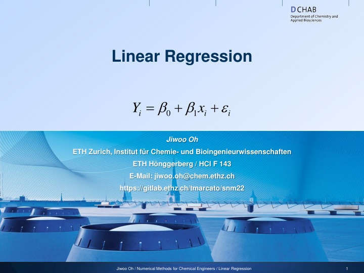
Linear Regression = + + Y x 0 1 i i i Jiwoo Oh ETH Zurich, Institut f r Chemie- und Bioingenieurwissenschaften ETH H nggerberg / HCI F 143 E-Mail: jiwoo.oh@chem.ethz.ch https://gitlab.ethz.ch/tmarcato/snm22 Jiwoo Oh / Numerical Methods for Chemical Engineers / Linear Regression 1
Linear regression model As inputs for our model we use two vectors x and Y, where xiis the i-th observation Yiis the i-th response The model reads: or i Y x Y = + + = + + x 0 1 0 1 i i At this point, we make a fundamental assumption: The errors are mutually independent and normally distributed with mean zero and variance 2: N 2 0, i As outputs from our regression we get estimated values for the regression parameters: , A regression is called linear if it is linear in the parameters! 0 1 Jiwoo Oh / Numerical Methods for Chemical Engineers / Linear Regression 2
The errors Since the errors are assumed to be normally distributed, the following is true for the expectation values and variance of the model responses ( ) ( 0, var( ) var( i Y = = + + + + = = + = = ) E Y E x x 0 1 0 1 i i i i i N i 2 ) var( ) x 0 1 i i i ( ) = + E Y 1 i x 0 Y 2 , i i Jiwoo Oh / Numerical Methods for Chemical Engineers / Linear Regression 3
Example: Boiling Temperature and Pressure Jiwoo Oh / Numerical Methods for Chemical Engineers / Linear Regression 4
Parameter estimation 1 x Y 1 1 = = , X Y 1 x Y N N obs obs = confidence interval Jiwoo Oh / Numerical Methods for Chemical Engineers / Linear Regression 5
Residuals Outlier N obs = 0 i = 1 i N obs = 0 x i i = 1 i Jiwoo Oh / Numerical Methods for Chemical Engineers / Linear Regression 6
Removing the Outlier Jiwoo Oh / Numerical Methods for Chemical Engineers / Linear Regression 7
The LinearModel and dataset classes Matlab 2012 features two classes that are designed specifically for statistical analysis and linear regression dataset creates an object that holds data and meta-data like variable names, options for inclusion / exclusion of data points, etc. LinearModel is constructed from datasets or X, Y pairs (as with the regress function) and a model description automatically does linear regression and holds all important regression outputs like parameter estimates, residuals, confidence intervals etc. includes several useful functions like plots, residual analysis, exclusion of parameters etc. Jiwoo Oh / Numerical Methods for Chemical Engineers / Linear Regression 8
Classes in Matlab Classes define a set of properties (variables) and methods (functions) which operate on those properties This is useful for bundling information together with ways of treating and modifying this information When a class is instantiated, an object of this class is created which can be used with the methods of the class, e.g. mdl = LinearModel.fit(X,Y); Properties can be accessed with the dot operator, like with structs (e.g. mdl.Coefficients) Methods can be called either with the dot operator, or by having an object of the class as first input argument (e.g. plot(mdl) or mdl.plot()) Jiwoo Oh / Numerical Methods for Chemical Engineers / Linear Regression 9
Working with LinearModel and dataset First, we define our observed and measured variables, giving them appropriate names, since these names will be used by the dataset and the LinearModel as meta-data Jiwoo Oh / Numerical Methods for Chemical Engineers / Linear Regression 10
Working with LinearModel and dataset Next, we construct the dataset from our variables Jiwoo Oh / Numerical Methods for Chemical Engineers / Linear Regression 11
Working with LinearModel and dataset After defining the relationship between our data (a model), we can use the dataset and the model to construct a LinearModel object This will automatically fit the data, perform residual analysis and much more Jiwoo Oh / Numerical Methods for Chemical Engineers / Linear Regression 12
LinearModel: Plot Now that we have the model, we have many analysis and plotting tools at our disposal LogP vs. Temp 0.02 0 -0.02 -0.04 -0.06 LogP -0.08 Data Fit Confidence bounds -0.1 -0.12 -0.14 -0.16 -0.18 90 92 94 96 98 100 102 Temp Jiwoo Oh / Numerical Methods for Chemical Engineers / Linear Regression 13
Linear Model: Tukey-Anscombe Plot Plot residuals vs. fitted values; These should be randomly distributed around 0 14x 10 -3 Plot of residuals vs. fitted values Outlier? 12 10 8 Residuals 6 4 2 0 -2 -4 -0.16 -0.14 -0.12 -0.1 -0.08 Fitted values -0.06 -0.04 -0.02 0 0.02 Jiwoo Oh / Numerical Methods for Chemical Engineers / Linear Regression 14
LinearModel: Cooks Distance The Cook s distance measures the effect of removing one measurement from the data Case order plot of Cook's distance 0.5 0.45 0.4 0.35 Cook's distance 0.3 0.25 0.2 0.15 0.1 0.05 0 0 2 4 6 8 10 12 14 16 18 Row number Jiwoo Oh / Numerical Methods for Chemical Engineers / Linear Regression 15
Linear Model: Removing the Outlier After identifying an outlier, it can be easily removed -3 Case order plot of Cook's distance Plot of residuals vs. fitted values LogP vs. Temp 1.5x 10 0.02 0.5 0.45 0 1 0.4 -0.02 0.5 0.35 -0.04 0 Cook's distance 0.3 Residuals -0.06 0.25 -0.5 LogP -0.08 0.2 Data Fit Confidence bounds -1 -0.1 0.15 -1.5 -0.12 0.1 -2 -0.14 0.05 -0.16 -2.5 0 -0.16 90 0 -0.14 2 92 -0.12 4 94 6 -0.1 -0.08 8 96 -0.06 10 -0.04 98 12 -0.02 14 100 16 0 102 18 0.02 Row number Fitted values Temp Jiwoo Oh / Numerical Methods for Chemical Engineers / Linear Regression 16
Multiple linear regression Approximate model 1 Y x x 1 1,1 1, 1 0 0 p = + = + Y X 1 Y x n p x ,1 , 1 n n n 1 p Residuals = r Y Y Least squares ( ( ) ) 2 2 = = r Y Y T T min min X X X Y Jiwoo Oh / Numerical Methods for Chemical Engineers / Linear Regression 17
Assignment 1 The data file asphalt.dat (online), contains data from a degradation experiment for different concrete mixtures[1] The rutting (erosion) in inches per million cars (RUT) is measured as a function of viscosity (VISC) percentage of asphalt in the surface course (ASPH) percentage of asphalt in the base course (BASE) an operating mode 0 or 1 (RUN) percentage (*10) of fines in the surface course (FINES) percentage of voids in the surface course (VOIDS) [1] R.V. Hogg and J. Ledolter, Applied Statistics for Engineers and Physical Scientists, Maxwell Macmillan International Editions, 1992, p.393. Jiwoo Oh / Numerical Methods for Chemical Engineers / Linear Regression 18
Assignment 1 (Continued) 1. Find online the file readVars.m that will read the data file and assign the variables RUT, VISC, ASPH, BASE, RUN, FINES and VOIDS; You can copy and paste this script into your own file. Create a dataset using the variables from 1. Set the RUN variable to be a discrete variable Assuming your dataset is called ds, use ds.RUN = nominal(ds.RUN); Create a modelspec string To include multiple variables in the modelspec, use the plus sign How many dependent and independent variables does you problem contain? 2. 3. 4. 5. Fit your model (mdl1) using LinearModel.fit, display the model output and plot the model. Jiwoo Oh / Numerical Methods for Chemical Engineers / Linear Regression 19
Assignment 1 (Continued) 6. Which variables most likely have the largest influence? 7. Generate the Tukey-Anscombe plot. Is there any indication of nonlinearity, non-constant variance or of a skewed distribution of residuals? 8. Plot the adjusted responses for each variable, using the plotAllResponses function you can find online. What do you observe? 9. Try and transform the system by defining logRUT = log10(RUT); logVISC = log10(VISC); 10.Define a new dataset and modelspec using the transformed variables. Jiwoo Oh / Numerical Methods for Chemical Engineers / Linear Regression 20
Assignment 1 (Continued) 11. Fit a new model with the transformed variables and repeat the analysis from before (steps 6.-8.). 12. With the new model, try to remove variables that have a small influence. To do this systematically, use the function step, which will remove and/or add variables one at a time: mdl3 = step(mdl2, 'nsteps', 20); Which variables have been removed and which of the remaining ones most likely have the largest influence? Do you think variable removal is helpful to improve general conclusions (in other words avoid overfitting)? How could you compare the quality of the three models? Is the root mean squared error of help? How could you determine SST, SSR and SSE of your models (at least 2 options)? How could you improve the models? Think about synergic effects. Jiwoo Oh / Numerical Methods for Chemical Engineers / Linear Regression 21
