Logical Agents Acting Under Uncertainty

ECE469: Artificial Intelligence Probability

Acting under Uncertainty Many agents must often act under uncertainty due to partial observability or non-determinism Strictly speaking, if a logical agent cannot conclude that any particular cause of action will achieve its goal, it will be unable to act A logical agent may rely on a belief state, representing the set of all possible world states that it might be in It might be able to generate a contingency plan that handles every possibility However, the belief states and the contingency plans themselves may become arbitrarily large, and there might not be any plan that is guaranteed to achieve the goal The belief state of a rational agent also specifies the probabilities of all possible world states Book: "The right thing to do the rational decision therefore depends on both the relative importance of various goals and the likeliness that, and degree to which, they will be achieved." One real-world example dealing with uncertainty: Getting to the airport on time Another example: diagnosis in various domains (medicine, automobile repair, dentistry, etc.)

First-order Logic Doesnt Cut It Consider a dental patient with a toothache that needs to be diagnosed A logical agent might conclude that the patient has a toothache based on the following rule expressed using first-order logic (FOL): ? Symptom ?,Toothache Disease ?,Cavity That rule is wrong; not all patients with toothaches have cavities Perhaps we could try something more robust, such as: ? Symptom ?,Toothache Disease ?,Cavity Disease ?,GumDisease Disease ?,Abscess This rule is still probably wrong, because we wouldn t know all the possible causes of a toothache, and it also tells us nothing about the relative likelihoods of the various causes Maybe we could try going in the opposite direction: ?Disease ?,Cavity Symptom ?,Toothache This is still wrong, because not every cavity causes a toothache, and it doesn t help us with diagnosis anyway First-order logic fails for domains like this for at least three reasons, that our textbook refers to as: Laziness - it takes too much work to list all the rules and use the rules Theoretical ignorance - not everything is known; the science is not complete Practical ignorance - not all possible tests have been run on a patient

Probability Theory The agent's knowledge can only provide degrees of belief about relevant facts or sentences The main tool to deal with degrees of belief is probability theory According to our textbook, a probability of 0 or 1 represents the "unequivocal belief" that a sentence is either false or true (although the quoted phrase has been dropped from Ed. 4) All other probabilities lie between 0 and 1, representing intermediate degrees of belief Note that degrees of beliefs (probabilities) are different than degrees of truth A sentence expressing a fact is still either true or false, we just don't know for certain Fuzzy logic provides an alternate means of dealing with uncertainty in which values represent degrees of truth, but we will not discuss this further in this course Note: Not all sources agree with our textbook s definition of probability Our textbook uses what I would refer to as a Bayesian view of probability, as opposed to a frequentist view of probability (I'll discuss the distinction in class); both views are common in the literature Interpreting a probability as a degree of belief seemed unintuitive to me when I first encountered this concept However, I ve since concluded that both views of probability are potentially problematic, and I currently think that the Bayesian view is probably better suited to deal with most AI contexts

Possible Worlds In probability theory, the set of all possible worlds is called the sample space In AI, we can think of the sample space as containing all possible configurations of an agent s environment The possible worlds are mutually exclusive and exhaustive; for now, we'll assume that they form a discrete, countable set A probability model assigns each possible world a probability between 0 and 1 The sum of the probabilities assigned to all possible worlds must be 1 Probabilistic assertions and queries are usually about particular sets of possible worlds; in probability theory, each such set is called an event Note: I also find this definition of "event" unintuitive In sources that take a frequentist view of probability, an event may be defined as the outcome of a hypothetical experiment, which seems more intuitive to me

Propositions We will be assigning degrees of belief (i.e., probabilities) to propositions, i.e., assertions that something is true We can think of a proposition as a declarative sentence expressed in a formal language; it is either true or false, but we don't know with certainty Each proposition corresponds to an event containing the possible worlds for which the assertion is true For example, if we roll two dice, we might consider the proposition that the sum of the two dice is 11 For fair dice, we might calculate: P(Total = 11) = P((5,6)) + P((6,5)) = 1/36 + 1/36 = 1/18 More generally, the probability of a proposition, ?, is the sum of the probabilities of the possible worlds in which it holds: P ? = ? ?P(?)

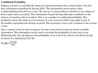
Prior and Conditional Probabilities Before any evidence is obtained, there is an unconditional probability, a.k.a. a prior probability (or just a prior), for every proposition An example of a prior probability is: P(Total = 11) After evidence is obtained that changes our degree of belief, we have a conditional probability, a.k.a. a posterior probability For example, if we know the first die has landed on 5, we might consider P(Total = 11 | Die1= 5) P(a | b) can be read as "the probability of a given b" Mathematically, conditional probabilities can be defined in terms of unconditional probabilities For any propositions a and b: P(a | b) = P(a ^ b) / P(b) We can rewrite this as the product rule: P(a ^ b) = P(a | b) * P(b)

Random Variables Variables in probability theory are called random variables; by convention, we will represent random variables with capitalized names Each random variable has a domain of values it can take on We will focus on three types of random variables: Boolean random variables: The domain of a Boolean random variable (e.g., Cavity) is <true, false> We can abbreviate the proposition Cavity = true as the lowercase name cavity; Cavity = false can be abbreviated as cavity Discrete random variables (Boolean is really a special case of discrete): They take on values from a countable domain; e.g., Weather may have the domain <sun, rain, cloud, snow> Values in the domain must be mutually exclusive and exhaustive; if there is no confusion, you can abbreviate Weather = snow with snow Discrete random variables can have infinite domains (e.g., the integers) Continuous random variables: These take on values that are real numbers The domain can be the entire real number line or an interval; e.g., [0, 1]

Probability Distributions Sometimes we want to express the probabilities of all possible values of a random variable When dealing with a discrete random variable with a finite domain, this can be expressed as a vector For example, suppose that P(Weather = sun) = 0.6, P(Weather = rain) = 0.1, P(Weather = cloud) = 0.29, and P(Weather = snow) = 0.01 We can write this as P(Weather) = <0.6, 0.1, 0.29, 0.01>, assuming we know which dimension of the vector corresponds to each possible value (note the boldfaced P , since it is a distribution, not a single probability) This defines a probability distribution for the random variable Weather Probability distributions for discrete, finite domains are also called categorical distributions For a continuous random variable, it is not possible to write out the distribution as a vector, but we can express a probability density function A joint probability distribution specifies the probabilities of all possible combinations of values for a set of random variables The full joint probability distribution specifies probabilities for all combinations of all random variables used to describe the world we are dealing with If all the random variables are discrete with finite domains, then this can be specified by a table (there is an example on the next slide)

Full Joint Probability Distribution Example

The Axioms of Probability The axioms of probability are often listed as: All probabilities range from 0 to 1, inclusive The sum of the probabilities of all possible worlds is 1 For any set of mutually exclusive possible worlds, ?, the probability of ? is: P ? = ???P(?) From these, we can derive the inclusion-exclusion principle: P ? ? = P ? + P ? P ? ? I add: Our textbook groups the first two axioms of probability listed above, together with the inclusion-exclusion principal, as Kolmogorov s axioms However, I think this is unusual Some sources define Kolmogorov's axioms to be the same as the three axioms of probability listed above In general, not all sources agree on exact definitions of the axioms of probability or Kolmogorov's axioms

Inconsistent Beliefs Consider the following beliefs (example from textbook): P(a) = 0.4, P(b) = 0.3, P ? ? = 0.0, P ? ? =0.8 Clearly these statements are inconsistent If we define probabilities to be "degrees of belief", however, why can t an agent hold them? The book discusses an example which basically explains that inconsistent beliefs can lead to gambling losses I personally do not find that argument convincing; none-the-less, the set of beliefs stated above is clearly not rational

Computing Prior Probabilities Remember that the probability of a proposition is equal to the sum of the probabilities of the possible worlds in which it holds This leads to a simple method of computing the probability of any proposition given a full joint distribution, when such a distribution is available Here are a couple of examples of computing prior probabilities given the full joint distribution we looked at earlier Example 1: P(cavity toothache) = 0.108 + 0.012 + 0.072 + 0.008 + 0.016 + 0.064 = 0.28 Example 2: P(cavity) = 0.108 + 0.012 + 0.072 + 0.008 = 0.2 The second example is an example of marginalization, or summing out, which basically means summing up all probabilities of a row or column in the table Marginalization can be generalized for distributions as follows: ? ? = ?? ?,? = ? , where Y and Z are sets of variables We can rewrite this using the product rule for distributions as follows: ? ? = ?? ?|? P ? Written in this form, this is called conditioning; note that the last term is not a distribution

Probabilistic Inference Probabilistic inference involves the computation of conditional probabilities for query propositions given observed evidence Recall that conditional probabilities are defined in terms of prior probabilities, so these can also be computed from a full join distribution Example 1: ? ?????? | ???? ?? ? =? ?????? ???? ?? ? Example 2: ? ?????? | ???? ?? ? =? ?????? ???? ?? ? 0.108+0.012 = 0.108+0.012+0.016+0.064= 0.6 0.016+0.064 0.108+0.012+0.016+0.064= 0.4 ? ???? ?? ? = ? ???? ?? ? Note that the two probabilities above add up to 1, which must be the case

Normalization Constant In the previous two equations, the denominator is the same; i.e., both numerators are multiplied by 1 / P(toothache) We can view this as a normalization constant, For our current example case, we can thus write: P(Cavity | toothache) = P(Cavity, toothache) = [P(Cavity, toothache, catch) + P(Cavity, toothache, catch)] = [<0.108, 0.016> + <0.012, 0.064>] = <0.12, .08> = <0.6, 0.4> Note that the capitalized tokens represent random variables, and the lowercase tokens represent abbreviations for specific propositions Remember that when P is boldfaced, it represents a distribution For the final step in the computation, we can either compute the normalization constant, or we can scale the values to sum to one

General Inference Procedure Let X be a single random variable for which we want to calculate the probability distribution given some observed evidence Let E be the set of evidence variables and e represent their observed values Let Y represent the remaining unobserved random variables We can compute: P(X|e) = P(X, e) = ? ??(?,?,?) This is easy if we have a full joint probability distribution in the form of a table, but typically, we won t Even if all random variables are Boolean, n random variables would have a space requirement of 2n

Independence Now, we will introduce Weather to the world of Cavity, Catch, and Toothache Suppose we want to calculate P(toothache, catch, cavity, cloud) Using the product rule, we can equate this to P(cloud | toothache, catch, cavity) P(toothache, catch cavity) It seems reasonably safe to conclude that the weather is not influenced by a patient s dental conditions, and vice versa; with these assumptions, we can conclude that P(cloud | toothache, catch, cavity) = P(cloud) Based on this, we can deduce that P(toothache, catch, cavity, cloud) = P(cloud) P(toothache, catch, cavity) We can generalize this to distributions: P(Toothache, Catch, Cavity, Weather) = P(Weather | Toothache, Catch, Cavity) P(Toothache, Catch, Cavity) = P(Weather) P(Toothache, Catch, Cavity) This works because the weather is (presumably) independent of a patient s dental conditions; the property is known as independence (a.k.a. marginal independence or absolute independence) The definition of independence between random variables X and Y can be written in any of these three ways: P(X | Y) = P(X) or P(Y | X) = P(Y) or P(X, Y) = P(X)P(Y) Independence assertions are usually based on knowledge of the domain If the complete set of random variables can be divided into independent subsets, the full joint distribution can be factored into separate joint distributions on each subset (examples are shown on the next slide)

Factoring Examples

Bayes Rule Recall the product rule in its simplest form: P(a ^ b) = P(a | b) * P(b) This can also be written as: P(a ^ b) = P(b | a) * P(a) Equating the two right-hand sides and dividing by P(a) gives: P ?|? =P ?|? P(?) P(?) This equation is known as Bayes rule (a.k.a. Bayes law or Bayes theorem) Book: "This simple equation underlies most general modern AI systems for probabilistic inference." We can generalize this for distributions as follows: ? ?|? =? ?|? ?(?) ?(?)

Bayes Rule Example Suppose a doctor knows these facts: The disease meningitis causes a patient to have a stiff neck in 70% of cases Approximately 1 out of 50,000 patients have meningitis (this is a prior probability) Approximately 1 out of 100 patients have stiff necks (also a prior probability) We can express these facts as: P(s | m) = 0.7, P(m) = 1/50,000, P(s) = 0.01 I add: Strictly speaking, the first fact above should really be stated "70% of patients with meningitis have stiff necks"; some of them may have stiff necks for some other reason! We want to diagnose the patient with a stiff neck; i.e., to determine if they have meningitis We can use Bayes rule as follows: P ?|? =P ?|? P(?) P(?) 0.01 150000 0.7 = = 0.0014

Why is Bayes Rule Useful? Bayes rule is useful when we have estimates of the right-hand probabilities and we need to estimate the left-hand probability Let s think about this in relation to the previous example The doctor may know that a stiff neck implies meningitis 0.14% of the time; this is an example of diagnostic knowledge In practice, diagnostic knowledge is often more fragile than causal knowledge For example, the percentage of times that a patient with a stiff neck has meningitis, P(m | s), could change during an epidemic of meningitis However, P(s | m) would presumably not change, because it reflects the way that meningitis works Probabilistic information is often available in the form P(effect | cause), and these values are unlikely to change

Combining Evidence Now let s say a patient goes to the dentist, and the dentist notes the following two facts: The patient has a toothache The dentist s stick with a metal hook gets caught on the patient s tooth The dentist wants to calculate the probabilities that the patient does (or does not) have a cavity Note: I realize that, in reality, a dentist can check with their little mirror, or rely on x-rays, so we are taking this example with a grain of salt We want to calculate: P(Cavity | toothache ^ catch) Given the values in our full joint distribution, this becomes: P(Cavity | toothache ^ catch) = <0.018, 0.016> <0.871, 0.129> However, in practice, we do not typically have a full joint distribution; it is not feasible for real-world problems with many variables

Conditional Independence We can apply Bayes rule to the multiple-variable case and obtain: P(Cavity | toothache ^ catch) = P(toothache ^ catch | Cavity) P(Cavity) To finish this, we would need to have an estimate of the conditional probability of toothache ^ catch for each value of Cavity This would be simpler if Toothache and Catch were independent; if so, we could write: P(toothache ^ catch | Cavity) = P(toothache | Cavity) P(catch | Cavity) However, Toothache and Catch are clearly not independent; e.g., if the hook catches, a cavity is more likely, making a toothache more likely Fortunately, we can make a less strict assumption, and still use the same simplification; namely, Toothache and Catch are conditionally independent given Cavity In this case, that means that once we know about the presence or absence of a cavity, knowing the value of Toothache or Catch provides no additional evidence for the other Conditional independence assertions are more common in practice than absolute independence, and they allow probability systems to scale up The definition of conditional independence of random variables X and Y given random variable Z can be written in these three ways: P(X | Y, Z) = P(X | Z) or P(Y | X, Z) = P(Y | Z) or P(X, Y | Z) = P(X | Z) P(Y | Z)

Nave Bayes A commonly occurring pattern: A single cause directly influences several effects, all of which are conditionally independent given the cause Using what we learned about conditional independence, we can write: ? ? ?????,??????1, ,???????= ?(?????) ? ????????????) ?=1 This is called a na ve Bayes model The word "na ve" is used because this often relies on a simplifying assumption That is, the effects may not truly be conditionally independent of each other given the cause, but it is close enough such that the equation is still useful We will come back to this when we discuss Bayesian learning as part of our machine learning unit of the course