Low-Frequency Properties and Parameterization of Layered Medium - ORT Interpretation
Explore the low-frequency properties of a layered medium, including ORT stiffness coefficients, system matrix, upscaling techniques, and the BCH series. Understand dispersion in terms of ORT parameters and zero-frequency approximation for physical mediums. Discover insights by Alexey Stovas and IGP from NTNU.

Download Presentation

Please find below an Image/Link to download the presentation.
The content on the website is provided AS IS for your information and personal use only. It may not be sold, licensed, or shared on other websites without obtaining consent from the author. If you encounter any issues during the download, it is possible that the publisher has removed the file from their server.
You are allowed to download the files provided on this website for personal or commercial use, subject to the condition that they are used lawfully. All files are the property of their respective owners.
The content on the website is provided AS IS for your information and personal use only. It may not be sold, licensed, or shared on other websites without obtaining consent from the author.
E N D
Presentation Transcript
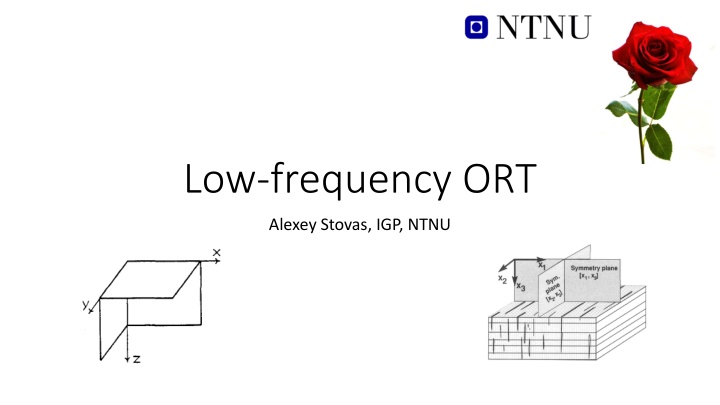
Low-frequency ORT Alexey Stovas, IGP, NTNU
OUTLINE Low-frequency properties of layered medium ORT medium and parameterization BCH series for ORT Eigenvalues, multipliers and frequency dependent velocities Interpretation of dispersion in terms of ORT parameters Conclusions
Low-frequency properties of the medium Zero- and infinite-frequency limits Given frequency w=w0 (non-physical medium) Low-frequency approximation + =
ORT: stiffness coefficient matrix c c c c c c 11 12 13 22 23 33 = C c 44 c 55 c 66 ( ) ij c ( ) , , , , , , , , v v Tsvankin, 1997 0 0 1 2 1 2 3 1 2 P S
System matrix for ORT 1 c c c c 13 23 p p 1 2 c p p 33 c c c c 33 33 1 2 M 0 N 1 = = = A N 13 p s s M 0 p 1 11 12 1 0 c 33 55 1 23 p s s 0 p 2 12 22 2 c 33 44 2 13 2 23 c c 13 23 c c c c c = + = + = + 2 1 2 2 2 2 2 1 , , . s c p c p s c c p p s c p c p 11 11 66 12 12 66 1 2 22 22 66 33 33 33
Upscaling (replacement of Schoenberg-Muir) = A A 1 c c c c 2 2 B B B B B B = = = , , , 13 23 B B B = + = + = , , , 2 B 3 c B c B B c 2 1 2 3 c 11 7 12 8 6 13 33 33 33 1 1 1 B 1 1 1 2 3 B B B B = = = , , , = + = = B B B c , , , 3 c B c c 4 5 6 66 22 9 23 33 c c 44 55 1 1 1 1 B 1 B 2 13 2 23 c c 13 23 c c c c c = = = , , . c c c B = = + = , , B c B c c B c 44 55 66 6 7 11 8 12 66 9 22 4 5 33 33 33 Zero-frequency limit
The BCH series ( ) ( ) ( ) 2 = + i H + i H + A F F F ... 0 1 2 Roganov and Stovas, 2012
The BCH series ( ) = + F A A 1 , 0 1 2 1 2 1 12 ) ( = F A A 1 , , 1 2 1 ) ( ( ) = + F A A A A A A 1 1 , , , , , 2 2 2 1 1 1 2 [x,y] is a commuting operator is a volume fraction Roganov and Stovas, 2012
The BCH series M N M N 0 2 1 1 2 = A A , , 2 1 N M N M 0 2 1 1 2 M M N M M N 0 2 1 2 2 2 1 = A A A , , 2 , 2 2 1 N M N N M N 0 2 2 1 2 1 2 M M N M M N 0 1 2 1 1 1 2 = A A A , , 2 . 1 1 2 N M N N M N 0 1 1 2 1 2 1 Roganov and Stovas, 2012
+ m m m m m m = 2 , m 2 1 Weak contrast 2 1 = m 2 1 a a a Isotropic background Weak contrast in elastic and anisotropy parameters 1 v ( ) ( ) 1 2 1 2 2 0 2 0 p p p p 1 2 2 P M 0 0 1 2 0 0 ( ) ( ( ) ) ( ) ( ) 1 v 0 = A = 1 2 1 4 1 2 3 4 2 0 2 0 2 1 2 S 2 2 2 S 2 S 2 0 N p p v p v p p v = M 0 p 0 1 0 0 0 0 1 2 0 0 0 1 2 S N 0 ( ) 0 0 ( ) ( ) 0 1 2 3 4 2 0 2 S 2 0 2 1 2 S 2 0 2 2 2 S 1 4 1 2 p p p v p v p v 1 v 2 0 1 2 0 0 0 0 0 p 2 2 S 0 0 ( ) ( ) 2 2 2 P 2 S 2 1 2 2 2 2 2 2 3 2 1 2 2 , , , , , , , , , o o d dv dv 1 = = + + + 2 A A A A , A A 1 0 Matrix series with respect to contrast 2 , A A 2 0
Weak contrast ( ) ( ) 2 = 1 2 + + 2 0 F A o A A 0 ) ( 11 6 = F 1 , , A A 1 0 ( ) ( ) = 1 2 + F A , , , , , A A A A A 2 0 0 0
Weak contrast ( ) = + + A R R R Matrix series with respect to contrast 0 1 2 = R A , 0 0 ( )( 6 ) 1 2 1 ) ( ( ) ( ) 2 = 1 2 + i H i H R 1 , , , , A A A A A A 1 0 0 0 ( ) 1 ( ) 2 = + i H 2 R , , . A A A A 2 0 6 No second-order contrasts in dispersion terms!
Characteristic equation (eigenvalues) ( ) = A I det 0 q ( ) ( ) ( ) + + + = 6 4 2 0 q a q a q a 4 2 0
Characteristic equation (eigenvalues) ( ) = + + 2 j 2 j 2 2 3 2, q q H d o 0 j ( ) 2 2 2 1 3 ( ) ( ) 0 j ( ) 0 j ( ) 0 j ( ) 0 j = 1 d q k q A A I A 0 j j ( ) 0 j ( ) 0 j k = j
Characteristic equation (P-eigenvalues) ( ) 0 P ( ) 0 P k = P ( ( ) ( ( ) ) ( ) ( ) T ( ) 0 P ( ) 0 P ( ) 0 P ( ) 0 P = 1 2 + = 2 1 2 2 2 S , , , p p v p p 1 0 0 1 2 1 2 ) ( ) 0 P ( ) 0 P ( ) 0 P ( ) 0 P = , 2 , 2 0 P 0 P 2 S 0 P 2 S = q q p v q p v , 2 1 0 0 2 0 0 2 1 ( ) 0 P = 2 k q 0 P
Slowness surface dispersion P S1 S2 Frequency
P wave (down, up) S1 wave (down, up) S2 wave (down, up) ( ) ( ) e , , i p p = = 1 2 , , 0 0 p p 1 2 Multipliers p1=0.1 p2=0.1 p1=0.05 p2=0.2 p1=0.2 p2=0.05
Frequency-dependent phase velocity P-wave Phase velocity, km/s S1-wave S2-wave = = 0.1 p p s km 1 2 Frequency, Hz
Wave mode selection Trial series for dispersion coefficient: ( ) 2 ( ) 00 ( ) 20 ( ) 02 ( ) 40 ( ) 22 ( ) 04 j j j j j j = + + + + + + 2 1 2 2 4 1 2 1 2 2 4 2 j d a a p a p a p a p p a p o Three solutions for a00 that give the wave mode selection.
Quadratic form ( )( 4 0 3 P v = m D 2 2 1 ( ( ( ) , ( ( 2 ) , = = = = = + + + ) ( 00 ) m m , , , , , , , , v v v v 2 qP = + , a v 20 2 02 1 1 2 S P S P P ) ) m m , , , , , , , , v v v v 40 2 2 04 1 2 1 1 S P S P ( ) ) 2 2 m , , , , , . v v 1 ( 20 ) ( 2 ) 22 1 1 2 3 2 S P qP qP T m , a 20 20 2 S 12 v 0 ( ) 2 2 1 ( 02 ) ( 2 ) qP qP = T m D m , a 02 02 2 S 12 v 0 ( 12 ) 2 2 1 ( 40 ) ( 4 ) qP qP = T m D m , a 40 40 2 0 ( 12 ) 2 2 1 ( 04 ) ( 4 ) qP qP = T m D m , a 04 04 2 0 D4 D2 ( ) 2 2 1 6 ( 22 ) ( 22 ) qP qP = T m D m , a 22 22 2 0
Conclusions We derive the low frequency approximation for waves propagating in multi-layered orthorhombic model. The weak-contrast approximation is introduced. We show that the stop-bands are the result of interaction of different wave modes (P, S1 and S2). The stop-bands are illustrated by multipliers. By defining the low-frequency effective anisotropic parameters, we perform the sensitivity analysis for intrinsic anisotropy parameters.


")


")
")
")

")