Machine Learning Basics: Observations and Predictions
Start with a space of observations and targets to understand how observations determine targets in machine learning. Explore probabilistic framing, prediction functions, loss functions, and linear regression to create predictive models for various data sets and problems

Download Presentation

Please find below an Image/Link to download the presentation.
The content on the website is provided AS IS for your information and personal use only. It may not be sold, licensed, or shared on other websites without obtaining consent from the author.If you encounter any issues during the download, it is possible that the publisher has removed the file from their server.
You are allowed to download the files provided on this website for personal or commercial use, subject to the condition that they are used lawfully. All files are the property of their respective owners.
The content on the website is provided AS IS for your information and personal use only. It may not be sold, licensed, or shared on other websites without obtaining consent from the author.
E N D
Presentation Transcript
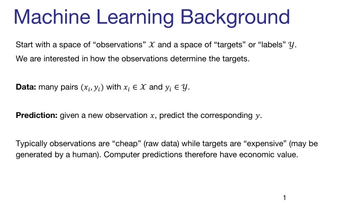
Machine Learning Background Start with a space of observations ? and a space of targets or labels ?. We are interested in how the observations determine the targets. Data: many pairs (??,??) with ?? ? and ?? ?. Prediction: given a new observation ?, predict the corresponding ?. Typically observations are cheap (raw data) while targets are expensive (may be generated by a human). Computer predictions therefore have economic value. 1
Prediction Problems Observation Space ?: Target Space ?: Images Image class: cat , dog etc. Images Caption: kids playing soccer Face Images User s identity Natural Images Stylized Images (e.g. cartoons) Signals of Human Speech Text transcript of the speech Sentence in English Translation into Spanish Demographic info: age, income Other info: education, employment Diet, lifestyle Risk of Heart Disease 2
Probabilistic Framing We assume that ? and ? are samples of random variables ? and ?. These random variables have a joint distribution ?(?,?). For prediction, we want at least the conditional distribution ?(?|?), so we can determine the distribution of targets ? given an observation ?. An approximation ?(?|?) to the true distribution ?(?|?) is called a model. The goal of machine learning is to construct models that are: 1. Computable (and perhaps simple, efficient) 2. Provide label predictions that are close to those from the true distribution ?(?|?) 3
Prediction Functions We can simplify the modeling task by making a strong assumption about the model ?(?,?), namely that ? = ?(?), i.e. ? takes a single value given ?. Examples: Linear regression, y = ?(?) is a linear function, and ? is a real value. Classifiers (SVM, random forest etc.), ? = ?(?) is the predicted class of ?, and ? {1, ,?} is the class number. 4
Loss Functions A loss function measures the difference between a target prediction and target data value. For instance: squared loss ?2 ?,? data pair. ? ?2where ? = ?(?) is the prediction, (?,?) is the = 5
Linear Regression Simplest case, ? = ? ? = ?? + ? with ? a real value, and real constants ? and ?. The loss is the squared loss ?2 ?,? ? ?2 = ? Data (?,?) pairs are the blue points. The model is the red line. ? ? ? 6
Linear Regression The total loss across all points is ? 2 ? = ?? ?? ?=1 ? 2 = ???+ ? ?? ?=1 We want the optimum values of ? and ?, and since the loss is differentiable, we set ?? ??= 0 and ?? ??= 0 7
Linear Regression We want the loss-minimizing values of ? and ?, so we set ? ? ? ?? ??= 0 = 2? 2+ 2? ?? ?? 2 ???? ?=1 ?=1 ?=1 ? ? ?? ??= 0 = 2? ?? + 2?? 2 ?? ?=1 ?=1 Two linear equations in ? and ?, easily solved. The model ? ? = ?? + ? with these values is the unique minimum-loss model. Aside: the least-squares loss is convex, making this work. 8
Multivariate Linear Regression This time, ? ?and ? ?, and the model is ? = ?? for a ? ? matrix ?. We assume the last coordinate of each ? vector is 1. Then the last column of ? acts as the bias vector ? we had before, simplifying the model. The loss function is ? ? ??? ?? ?(??? ??) 2= ? = ??? ?? ?? ?=1 ?=1 11
Multivariate Linear Regression We want to optimize ? with respect to the model matrix ?, so this time we need a gradient: ??? = 0 - we are treating the loss as a function ?(?) of the matrix ?. 12
Aside: Gradients When we write ???(?), we mean the vector of partial derivatives: ? ?? ??11 ?? ??12 ?? ??21 ?? ??22 ??? ? = , , , ?? ??11measures how fast the loss changes vs. change in ?11. Where When ??? ? i.e. the loss is not changing in any direction. = 0, it means all the partials are zero. Thus we are at a local optimum (or at least a saddle point). 13
Logistic Regression Setup: This time ? is an m-dimensional binary vector, i.e. ? {0,1}?, it could be the pixels in a binary image. The target values ? will also be binary, ? {0,1}, but our prediction ? = ?(?) will actually be a real value in the interval [0,1]. We can apply a threshold ? > ?? ??? ???later to get a class assignment to {0,1} The target class could be cat . The data are pairs (?,?) of images and labels, and ? = 1 means ? is a cat image, while ? = 0 means ? is no cat. Think of ? = ?(?), the output of our model, as being the probability that the image ? is cat. 14
Logistic Regression Let ? ?be a weight vector (the logistic model). Then 1 ? ? = 1 + exp ??? Is the probability that the output should be cat . We can write this as ? ? = ?(???) where ? ? = 1/ 1 + exp ? is the logistic function: ? ? ? 15
Loss for Logistic Regression We could use e.g. the squared loss between ? and ? = ?(?), but there are more natural (and effective) choices. Its based on our assumption that ? = ?(?) is the probability that ? is in the target class. Under this assumption, we can compute the probability of correct classification, and maximize that. The probability of correct classification (for one input) is: ? if ? = 1 if ? = 0 true positive probability (true negative probability) ????????= 1 ? Which we can turn into a simple expression as: ????????= ? ? + (1 ?)(1 ?) 16
Cross-Entropy Loss We can use ????????as the loss for each observation: ????????= ? ? (1 ?)(1 ?) We could sum this over all observations and minimize it to maximize the algorithm s overall accuracy. This is sometimes done, and may give good results. But much more commonly we use the negative log of the probability of a correct result: log????????= ?log ? 1 ? log(1 ?) This is called Cross-Entropy Loss (? is the number of observations): ? ? = ??log ??+(1 ??)log 1 ?? ?=1 Cross entropy loss in this case is the negative log probability that every label is correct - since label errors are independent, we should multiply them to get the overall probability that everything is correct. Taking logs turns this product into a sum. 17
Cross-Entropy Loss More generally Cross-Entropy Loss compares a target distribution ??(now a vector over the possible values of ?, ? is still the observation number) with a model distribution ??. ? ?log ?? ? = ?? ?=1 Its straightforward to show that the loss is minimized when ??= ??, i.e. the predicted probability should match the observed probabilities of the labels on the data. 18
Logistic Regression Is there something special about the logistic function 1 ? ? = 1 + exp ??? or would any other sigmoid function work? 19
Logistic Regression Is there something special about the logistic function 1 ? ? = 1 + exp ??? or would any other sigmoid function work? Exercise: show that a logistic regression classifier can exactly learn a Na ve Bayes classifier. i.e. find weights ? such that ?(?) is the Na ve Bayes probability that ? is in the class. 20
Multi-Class Logistic Regression We again consider the one-versus-rest design because its scalable. We assume ? is an m-dimensional vector. It may be binary or real-valued. We would like ??(?) to estimate the probability that ? is in class ?. Assume again that we apply the ? ? linear weight vector ? to ?, and let ? = ??. We define: exp ?? ??? = exp ?1 + exp ?2 + + exp ?? Clearly ? So it acts as a probability ??(?) = 1 ?=1 21
Multiclass Logistic Regression (Softmax) The formula: exp ?? ??? = exp ?1 + exp ?2 + + exp ?? Is called a softmax of the vector (?1, ,??). The intuition for the name softmax is that if some ??is somewhat larger than the others, its exponential will dominate the sum, and the output will be close to (0, ,1, ,0) where the 1 is in the ?? position. But that s not very compelling. Is there a more convincing argument for this particular choice of function? 22


")