Machine Learning Foundations: Occam's Razor and Probabilistic Models

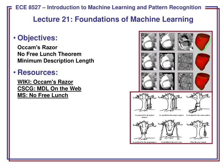
ECE 8443 Pattern Recognition ECE 8527 Introduction to Machine Learning and Pattern Recognition Lecture 21: Foundations of Machine Learning Objectives: Occam s Razor No Free Lunch Theorem Minimum Description Length Resources: WIKI: Occam's Razor CSCG: MDL On the Web MS: No Free Lunch

Introduction With such a wide variety of algorithms to choose from, which one is best? Are there any reasons to prefer one algorithm over another? Occam s Razor: if performance of two algorithms on the same training data is the same, choose the simpler algorithm. Do simpler or smoother classifiers generalize better? In some fields, basic laws of physics or nature, such as conservation of energy, provide insight. Are there analogous concepts in machine learning? The Bayes Error Rate is one such example. But this is mainly of theoretical interest and is rarely, if ever, known in practice. Why? ECE 8527: Lecture 21, Slide 1

Introduction In this section of the course, we seek mathematical foundations that are independent of a particular classifier or algorithm. Are there techniques that we can use to make any algorithm better? We will discuss techniques, such as jackknifing or cross-validation, that can be applied to any algorithm. We will also discuss some important philosophical points: No pattern classification method is inherently superior to any other. It is the type of problem, prior distributions and other application-specific information that determine which algorithm is best. Can we develop techniques or design guidelines to match an algorithm to an application and to predict its performance? Can we combine classifiers to get better performance? ECE 8527: Lecture 21, Slide 2

Important Consequences If one algorithm outperforms another, it is a consequence of its fit to the particular problem, not the general superiority of the algorithm. Thus far, we have estimated performance using a test data set which is sampled independently from the problem space. This approach has many pitfalls, since it is hard to avoid overlap between the training and test sets. We have learned about methods that can drive the error rate to zero on the training set. Hence, using held-out data is important. ECE 8527: Lecture 21, Slide 3

Probabilistic Models of Learning Consider a two-category problem where the training set, ?, consists of patterns, ??, and associated category labels, ?? = 1, for ? = 1, ?, generated by the unknown target function to be learned, ?(?), where ?? = ?(??). Let ? denote a discrete set of hypotheses or a possible set of parameters to be learned. Let (?) denote a particular set of parameters, (?) ?. Let ?( ) be the prior probability that the algorithm will produce after training. Let ?( |?) denote the probability that the algorithm will produce h when training on ?. Let ? be the error for a zero-one or other loss function. Where have we seen this before? (Hint: Relevance Vector Machines) ECE 8527: Lecture 21, Slide 4

No Free Lunch Theorem A natural measure of generalization is the expected value of the error given D: ? ?|? = ? ? 1 ? ? ? , (?) ?( |?)?(?|?) ,? ? ? where ?() denotes the Kronecker delta function (value of 1 if the two arguments match, a value of zero otherwise). The expected off-training set classification error when the true function ?(?) and the probability for the ?? candidate learning algorithm is ??( (?)|?) is: ??? ?,? = ? ?? ? 1 ? ? ? , (?)??( (?)|?) No Free Lunch Theorem: For any two learning algorithms ?1( |?) and ?2( |?), the following are true independent of the sampling distribution?(?)and the number of training points: 1. Uniformly averaged over all target functions, ?, ?1(?|?,?) ?2(?|?,?) = 0. 2. For any fixed training set ?, uniformly averaged over ?, ?1(?|?,?) ?2(?|?,?) = 0. 3. Uniformly averaged over all priors ?(?),?1(?|?,?) ?2(?|?,?) = 0. 4. For any fixed training set ?, uniformly averaged over ?(?), ?1(?|?,?) ?2(?|?,?) = 0. ECE 8527: Lecture 21, Slide 5

Analysis The first proposition states that uniformly averaged over all target functions the expected test set error for all learning algorithms is the same: ? ? ? ?1? ?,? ?2? ?,? = 0 ? ? Stated more generally, there are no? and ? such that for all ?(?), ??(?|?,?) > ??(?|?,?). Further, no matter what algorithm we use, there is at least one target function for which random guessing Is better. The second proposition states that even if we know ?, then averaged over all target functions, no learning algorithm yields a test set error that is superior: ?1? ?,? ?2? ?,? = 0 ? The six squares represent all possible classification problems. If a learning system performs well over some set of problems (better than average), it must perform worse than average elsewhere. ECE 8527: Lecture 21, Slide 6

Algorithmic Complexity Can we find some irreducible representation of all members of a category? Algorithmic complexity, also known as Kolmogorov complexity, seeks to measure the inherent complexity of a binary string. If the sender and receiver agree on a mapping, or compression technique, the pattern ? can be transmitted as ? and recovered as ? = ?(?). The cost of transmission is the length of ?,|?|. The least such cost is the minimum length and denoted: ? = ????:? ? =?? . A universal description should be independent of the specification (e.g., the programming language or machine assembly language). The Kolmogorov complexity of a binary string ?, denoted ?(?), is defined as the size of the shortest program string ?, that, without additional data, computes the string ?: ? ? = ????:? ? =?? where ? represents an abstract universal Turing machine. Consider a string of ?1?. If our machine is a loop that prints 1?, we only need log2? bits to specify the number of iterations. Hence, ?(?) = ?(log2?). ECE 8527: Lecture 21, Slide 7

Minimum Description Length (MDL) We seek to design a classifier that minimizes the sum of the model s algorithmic complexity and the description of the training data, ?, with respect to that model: ? ,? = ? + ? ? ????? MDL Examples of MDL include: Measuring the complexity of a decision tree in terms of the number of nodes. Measuring the complexity of an HMM in terms of the number of states. We can view MDL from a Bayesian perspective: ? ? =? ? ? ? ? The optimal hypothesis, , is the one yielding the highest posterior: = ?????? ? ? ? =?????? ???2? + ???2? ? Shannon s optimal coding theorem provides a link between MDL and Bayesian methods by stating that the lower bound on the cost of transmitting a string ? is proportional to log2?(?). ECE 8527: Lecture 21, Slide 8

Summary Occam s Razor: simpler models generalize better. Cross-Validation: discussed our general goal of finding learning techniques that improve the performance of any machine learning algorithm. The No Free Lunch Theorem: If we average over all possible data sets, no algorithm is better or worse. What tends to differentiate algorithms are the degree to which their assumptions match the requirements of a specific problem. There is always some chance that some algorithm can produce a better result on a specific database one can get lucky from time to time. There is no general theory that guides the selection of the best algorithm, but we can do an exhaustive search. To demonstrate a fundamental improvement, one should measure performance on several substantially different tasks if superiority cannot be proved theoretically. This is difficult since it often takes significant expertise to develop a state of the art system on a given task. Algorithmic Complexity and Minimum Description Length: algorithms must be compared at the same degree of complexity. ECE 8527: Lecture 21, Slide 9