Master of Science in Business Analytics - Accelerated 7-Week Modules
INFS 6351 offers a comprehensive program in Business Analytics by Jerald Hughes. Learn to set up development platforms, collect data, run analyses, and create visualizations. Dive into hands-on R and Python scripting for statistics and business analytics. Start by gaining access to internet, UTRGV Blackboard, and basic Excel and Word skills. Join now to enhance your data analytics skills for business success."

Download Presentation

Please find below an Image/Link to download the presentation.
The content on the website is provided AS IS for your information and personal use only. It may not be sold, licensed, or shared on other websites without obtaining consent from the author.If you encounter any issues during the download, it is possible that the publisher has removed the file from their server.
You are allowed to download the files provided on this website for personal or commercial use, subject to the condition that they are used lawfully. All files are the property of their respective owners.
The content on the website is provided AS IS for your information and personal use only. It may not be sold, licensed, or shared on other websites without obtaining consent from the author.
E N D
Presentation Transcript
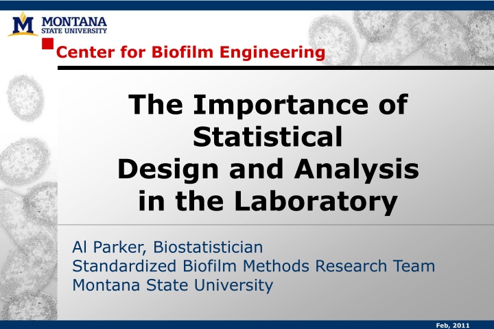
Center for Biofilm Engineering The Importance of Statistical Design and Analysis in the Laboratory Al Parker, Biostatistician Standardized Biofilm Methods Research Team Montana State University Feb, 2011
Standardized Biofilm Methods Laboratory Al Parker Lindsey Lorenz Marty Hamilton Darla Goeres Paul Sturman Diane Walker Kelli Buckingham- Meyer
What is statistical thinking? Data Experimental Design Uncertainty and variability assessment
What is statistical thinking? Data (pixel intensity in an image? log(cfu) from viable plate counts?) Experimental Design - controls - randomization - replication (How many coupons? experiments? technicians? labs?) Uncertainty and variability assessment
Why statistical thinking? Anticipate criticism (design method and experiments accordingly) Provide convincing results (establish statistical properties) Increase efficiency (conduct the least number of experiments) Improve communication
Why statistical thinking? Standardized Methods
Attributes of a standard method: Seven Rs Relevance Reasonableness Resemblance Repeatability (intra-laboratory) Ruggedness Responsiveness Reproducibility (inter-laboratory)
Attributes of a standard method: Seven Rs Relevance Reasonableness Resemblance Repeatability (intra-laboratory) Ruggedness Responsiveness Reproducibility (inter-laboratory)
Resemblance of Controls Independent repeats of the same experiment in the same laboratory produce nearly the same control data, as indicated by a small repeatability standard deviation. Statistical tool: nested analysis of variance (ANOVA)
Resemblance Example: MBEC 86 mm x 128 mm plastic plate with 96 wells Lid has 96 pegs
MBEC Challenge Plate 1 2 3 4 5 6 7 8 9 10 11 12 A 100 100 100 100 100 50:N N GC SC B 50 50 50 50 50 50:N N GC SC C 25 25 25 25 25 50:N N GC SC D 12.5 12.5 12.5 12.5 12.5 50:N N GC E 6.25 6.25 6.25 6.25 6.25 50:N N GC F 3.125 3.125 3.125 3.125 3.125 50:N N GC G 1.563 1.563 1.563 1.563 1.563 50:N N GC H 0.781 0.781 0.781 0.781 0.781 50:N N GC disinfectant neutralizer test control
Resemblance Example: MBEC Control Data: log10(cfu/mm2) from viable plate counts cfu/mm2 log(cfu/mm2) 5.71 5.95 5.78 5.48 5.59 5.33 4.93 5.63 row A 5.15 x 10⁵ B 9.01 x 10⁵ C 6.00 x 10⁵ D 3.00 x 10⁵ E 3.86 x 10⁵ F 2.14 x 10⁵ G 8.58 x 10⁴ H 4.29 x 10⁵ Mean LD= 5.55
Resemblance Example: MBEC Control LD 5.71 5.95 5.78 5.48 5.59 5.33 4.93 5.63 Mean LD Exp Row 1 1 1 1 1 1 1 1 SD A B C D E F G H 5.55 0.31 2 2 2 2 2 2 2 2 A B C D E F G H 5.41 5.71 5.54 5.33 5.11 5.48 5.33 5.41 5.41 0.17
Resemblance from experiment to experiment Mean LD = 5.48 Sr = 0.26 the typical distance between a control well LD from an experiment and the true mean LD
Resemblance from experiment to experiment The variance Sr2 can be partitioned: 2% due to between experiment sources 98% due to within experiment sources
Formula for the SE of the mean control LD, averaged over experiments 2 Sc = within-experiment variance of control LDs SE = among-experiment variance of control LDs nc = number of control replicates per experiment m = number of experiments 2 2 2 S S E c + SE of mean control LD = m nc m CI for the true mean control LD = mean LD tm-1 x SE
Formula for the SE of the mean control LD, averaged over experiments 2 Sc = 0.98 x (0.26)2 = 0.00124 SE = 0.02 x (0.26)2 = 0.06408 nc = 8 m = 2 2 0.06408 0.00124 = 0.1792 + SE of mean control LD = 2 8 2 95% CI for the true mean control LD = 5.48 12.7 x 0.1792 = (3.20, 7.76)
Resemblance from technician to technician Mean LD = 5.44 Sr = 0.36 the typical distance between a control well LD and the true mean LD
Resemblance from technician to technician The variance Sr2 can be partitioned: 0% due to technician sources 24% due to between experiment sources 76% due to within experiment sources
Repeatability Independent repeats of the same experiment in the same laboratory produce nearly the same data, as indicated by a small repeatability standard deviation. Statistical tool: nested ANOVA
Repeatability Example Data: log reduction (LR) LR = mean(control LDs) mean(disinfected LDs)
Repeatability Example: MBEC Control LD 5.71 5.95 5.78 5.48 5.59 5.33 4.93 5.63 Mean LD Exp Row 1 1 1 1 1 1 1 1 SD A B C D E F G H 1 100 2 100 3 100 4 100 5 100 6 50:N 7 N 8 GC 9 10 11 12 SC A 50 50 50 50 50 50:N N GC SC B 5.55 0.31 25 25 25 25 25 50:N N GC SC C 12.5 12.5 12.5 12.5 12.5 50:N N GC D 6.25 6.25 6.25 6.25 6.25 50:N N GC E 3.125 3.125 3.125 3.125 3.125 50:N N GC F 2 2 2 2 2 2 2 2 A B C D E F G H 5.41 5.71 5.54 5.33 5.11 5.48 5.33 5.41 1.563 1.563 1.563 1.563 1.563 50:N N GC G 0.781 0.781 0.781 0.781 0.781 50:N N GC H 5.41 0.17
Repeatability Example: MBEC Control LD 5.71 5.95 5.78 5.48 5.59 5.33 4.93 5.63 Control Mean LD Col Disinfected 6.25% LD Disinfected Mean LD Exp 1 1 1 1 1 1 1 1 Row A B C D E F G H LR 1 2 3 4 5 4.67 4.41 4.33 4.59 4.54 5.55 4.51 1.04 2 2 2 2 2 2 2 2 A B C D E F G H 5.41 5.71 5.54 5.33 5.11 5.48 5.33 5.41 1 2 3 4 5 4.78 2.71 3.48 3.23 1.82 5.41 3.20 2.21 Mean LR = 1.63
Repeatability Example Mean LR = 1.63 Sr = 0.83 the typical distance between a LR for an experiment and the true mean LR
Formula for the SE of the mean LR, averaged over experiments 2 Sc = within-experiment variance of control LDs Sd = within-experiment variance of disinfected LDs SE = among-experiment variance of LRs nc = number of control replicates per experiment nd = number of disinfected replicates per experiment m = number of experiments 2 2 2 2 2 S S S E d c + + SE of mean LR = m nd m nc m
Formula for the SE of the mean LR, averaged over experiments 2 Sc = within-experiment variance of control LDs Sd = within-experiment variance of disinfected LDs SE = among-experiment variance of LRs nc = number of control replicates per experiment nd = number of disinfected replicates per experiment m = number of experiments 2 2 CI for the true mean LR = mean LR tm-1 x SE
Formula for the SE of the mean LR, averaged over experiments Sc2 = 0.00124 Sd2 = 0.47950 SE2 = 0.59285 nc = 8, nd = 5, m = 2 0.59285 0.00124 0.47950 SE of mean LR = = 0.5868 + + 2 8 2 5 2 95% CI for the true mean LR = 1.63 12.7 x 0.5868 = 1.63 7.46 = (0.00, 9.09)
How many coupons? experiments? 0.59285 0.00124 0.47950 + + margin of error= tm-1 x m nd m nc m no. control coupons (nc): no. disinfected coupons (nd): no. experiments (m) 2 3 4 6 10 100 2 2 3 3 5 5 8 5 12 12 8.20 2.27 1.45 0.96 0.65 0.18 7.80 2.15 1.38 0.91 0.62 0.17 7.46 2.06 1.32 0.87 0.59 0.16 7.46 2.06 1.32 0.87 0.59 0.16 7.16 1.97 1.27 0.84 0.57 0.16
Responsiveness A method should be sensitive enough that it can detect important changes in parameters of interest. Statistical tool: regression and t-tests
Responsiveness Example: MBEC 1 2 3 4 5 6 7 8 9 10 11 12 A: High Efficacy A 100 100 100 100 100 50:N N GC SC B 50 50 50 50 50 50:N N GC SC C 25 25 25 25 25 50:N N GC SC D 12.5 12.5 12.5 12.5 12.5 50:N N GC E 6.25 6.25 6.25 6.25 6.25 50:N N GC F 3.125 3.125 3.125 3.125 3.125 50:N N GC G 1.563 1.563 1.563 1.563 1.563 50:N N GC H: Low Efficacy H 0.781 0.781 0.781 0.781 0.781 50:N N GC disinfectant neutralizer test control
Responsiveness Example: MBEC This response curve indicates responsiveness to decreasing efficacy between rows C, D, E and F
Responsiveness Example: MBEC Responsiveness can be quantified with a regression line: LR = 6.08 - 0.97row For each step in the decrease of disinfectant efficacy, the LR decreases on average by 0.97.
Summary Even though biofilms are complicated, it is feasible to develop biofilm methods that meet the Seven R criteria. Good experiments use control data! Assess uncertainty by SEs and CIs. When designing experiments, invest effort in more experiments versus more replicates (coupons or wells) within an experiment.