MATLAB Code Development for Nonlinear ODE BVP using Domain Decomposition

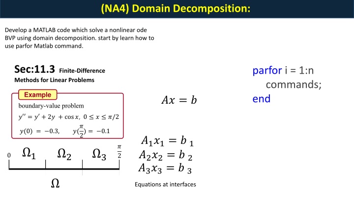
(NA4) Domain Decomposition: Develop a MATLAB code which solve a nonlinear ode BVP using domain decomposition. start by learn how to use parfor Matlab command. Sec:11.3 Finite-Difference Methods for Linear Problems parfor i = 1:n commands; end Example boundary-value problem ?? = ? ? = ? + 2? + cos?, 0 ? ?/2 ?(? ?(0) = 0.3, 2) = 0.1 ?1?1= ?1 ?2?2= ?2 ?3?3= ?3 ? 2 1 2 3 0 Equations at interfaces

(NA5) Newton-type methods with cubic convergence: Develop a MATLAB code which finds roots of a function. Start by reading the first three pages of the this paper "Homeier, H. H. H. "On Newton-type methods with cubic convergence." Journal of computational and applied mathematics 176.2 (2005): 425-432." Newton method by approximating the integral by trapezoidal approximation Potra and Pt k Frontini and Sormani considered the midpoint rule Weerakoon and Fernando rederived the Newton method

(NA6) Node ordering Study Use FDM to descritize Laplace equation then Develop a MATLAB code which assemble the matrix with different strategy of ordering then watch cpu time of the linear solver. Start by reading sec 11.3, 7.3 and search Red-black ordering. Sec:7.3 The Jacobi and Gauss-Siedel Iterative Techniques Red-black ordering Example boundary-value problem boundary-value problem ???+ ???+ ? ?? = ? 0,1 [0,1] ???+ ???+ ? ?? = ? 0,1 [0,1] 25 25 21 21 1 5 1 5 ?? = ? ?1?1= ?1

(NA7) Chebfun for Darcy's equation: Use Chebfun to solve 1D Darcy-Forchheimer equation. Start by getting the equation from A Block- Centered Finite Difference Method For The Darcy Forchheimer Model by Hongxing Rui and Hao Pan, SIAM J. Numer. Anal. vol. 50, no. 5, pp. 2612 2631" then solve it by chebfun. some links https://en.wikipedia.org/wiki/Chebfun http://www.chebfun.org/docs/guide/guide10.html DARCY FORCHHEIMER Nick Trefethen Chebfun is a system written in MATLAB that looks and feels like MATLAB, except that vectors and matrices become functions and operators. Whenever MATLAB has a discrete command, Chebfun aims to have the same command overloaded to execute a continuous analogue. For example, SUM(f) gives you the integral of a chebfun f over its interval of definition

(NA13) Preconditioning Technique Use Finite difference methods to solve 2ed or 4th order ode using two different scheme one with low order and the second with high order. Use the low order scheme matrix as a preconditioner to solve the linear system generated by the high order scheme. Start by reading sec 11.3 and search for preconditioning linear system or see these slides. Sec:11.3 Finite-Difference Methods for Linear Problems high order scheme Preconditioned linear system ? 1?? = ? 1? ?? = ? Example boundary-value problem ?? = ? ? = ? + 2? + cos?, 0 ? ?/2 low order scheme ?(? ?(0) = 0.3, 2) = 0.1 ?? = ? Faster convergence (less number of iterations)

(NA1) Multigrid Method Develop a MATLAB code which solve a linear 4th order BVP using two-grid method. Start by reading section 7.3 and iterative refinement in 7.5. You may consult the slides in here or A Multigrid Tutorial, Second Edition. Coarse Mesh ? ? = ? Sec:11.3 Finite-Difference Methods for Linear Problems Fine Mesh Example boundary-value problem ????= ?? ? ? = ? + 2? + cos?, 0 ? ?/2 ?(? ?(0) = 0.3, 2) = 0.1 high order scheme

(NA1) Multigrid Method Two-Grid Cycle Algorithm Remark: Ax = b = A x b 1) few GS iterations on the system h h h x Given an approximate: hx x Pre-smoothing step to obtain an approximate solution = T r r = b P A r We want to improve this approximate: 2) Compute the residual h h h 3) Restrict the residual Restriction step H h = = r e b x A x x (residual) = 4) Solve residual equation on coarse mesh A e r ProloCorrectio n step (error) H H H e = Pe = = x Prolongation step r r r = Ax A Ae A x x 5) Interpolate h = H e + x x ( ) 6) Update h h h = A x b 7) few GS iterations on the system h h h hx With initial approximate Post-smoothing step

(NA9) Numerical Comparison Study for RK and chepfun in chemical eng Select an IVP in chemical eng and solve it using RK and Chebfun. some links https://en.wikipedia.org/wiki/Chebfun http://www.chebfun.org/docs/guide/guide10.html Nick Trefethen if the rate of the reaction is r and if denote the concentration of compound A, . . . by CA, . . . , Chebfun is a system written in MATLAB that looks and feels like MATLAB, except that vectors and matrices become functions and operators. Whenever MATLAB has a discrete command, Chebfun aims to have the same command overloaded to execute a continuous analogue. For example, SUM(f) gives you the integral of a chebfun f over its interval of definition

Sec:11.3 Finite-Difference Methods for Linear Problems Example boundary-value problem The finite difference method for the linear second-order boundary- value problem ? = ? ? ? + ? ? ? + ?(?), ? ? ?, ? = ? + 2? + cos?, 0 ? ?/2 ?(? ?(0) = 0.3, 2) = 0.1 with ?(?) = ? and ?(?) = ?, ? ? = ? ??(???? + ? ????).

Sec:11.3 Finite-Difference Methods for Linear Problems Example 3 At the interior mesh points, xi, for i = 1:N, the differential equation is approximated as ( centeral diff ) boundary-value problem ? (??) = ? (??) + ??(??) + ????? ? = ? + 2? + cos?, 0 ? ?/2 ? = ?:? ?(? ?(0) = 0.3, 2) = 0.1 ?(??+?) ?(?? ?) ?? +?( 2) ?(??+?) ??(??) + ?(?? ?) ?? +?( 2) + ????? ??(??) + = ? = ?:? 1 we select an integer N N=3 ?(??+?) ?(?? ?) ?? ?(??+?) ??(??) + ?(?? ?) ?? + ????? ??(??) + divide the interval [a, b] into (N+1) equal subintervals 2 ??+? ???+ ?? ? ?? =??+? ?? ? ?? + ???+ ????? ??= ? + ? ? = 1:? + 1 Multiply by ?? and collect similar terms ? = ?:? = (? ?)/(? + 1) ??+?+ ??? ?? ? =? ?? ??+?+ ?? ? ????? ??????? ? = ?/? ? +? ?? ??+?+ ? ??+ ? ??+ ? ? ?? ?? ?= ??????? ?? ?? ?? ??= ?.? ??= ?.? ?? ?? ?? ?? ?? ?/? ? ??/? ??/? ?/?

Sec:11.3 Finite-Difference Methods for Linear Problems Example ? = ?:? We have the following: ? +? ?? ??+?+ ? ??+ ? ??+ ? ? boundary-value problem ?? ?? ?= ??????? ? = ? + 2? + cos?, 0 ? ?/2 ? +? ?? ??+ ? ??+ ? ??+ ? ? 4 ? = ? ?? ??= ??????? ?(? ?(0) = 0.3, 2) = 0.1 ? +? ?? ??+ ? ??+ ? ??+ ? ? ? = ? ?? ??= ??????? ? +? ?? ??+ ? ??+ ? ??+ ? ? ?? ??= ??????? ? = ? 5 Write in Matrix form and solve the system ? +? ?(??+ ?) ? +? = ??????? ?.?(? +? ?? ? ?? ??+ ? ??+ ? ??+ ??) ?? ?? ?? ? ? ? +? ?(??+ ?) ?? ?? ? +? ?? ??+ ? ??+ ? ??+ ? ? ?? ??= ??????? ? ? ?(??+ ?) ? ?? +? ??+ ? ??+ ? ? ?? ??= ??????? ?.?(? ? ??) ????? ?/? ?.?(? + ?) ????? ?/? ?? ? = ????? ?.?(? ?) ?? ?? ??= ?.? ?? ??= ?.? ?? ?? ?? ?? ?? ??/? ? ??/? ?/? ?/?

Sec:11.3 Finite-Difference Methods for Linear Problems Example ? +? boundary-value problem ?(??+ ?) ?? ? ????? ?/? ?.?(? + ?) ????? ?/? ?? ? ?? ?? ?? ? ? ? +? ? = ? + 2? + cos?, 0 ? ?/2 ?(??+ ?) ?? ?? = ?(? ????? ?.?(? ?) ? ? ?(0) = 0.3, 2) = 0.1 ?(??+ ?) ? ?? ?? ?? ?? ?? ?? ?? 2.3084 -0.8037 0 -0.5014 -0.1090 -0.1394 ?.???? ?.???? ?.???? -1.1963 2.3084 -0.8037 0 -1.1963 2.3084 = = ?(??/?) ?(??/?) ?(?/?) -0.2070 -0.3157 -0.2829 ?? ?? ?? ??= ?.? ??= ?.? ?? ?? ?? ?? ?? ?/? ? ??/? ??/? ?/?

Sec:11.3 Finite-Difference Methods for Linear Problems ? ? ? ? ?(??+ ?) ?? ? ????? ?.?(? + ?) ?? ?? ?? ? +? ? ? ????? ?/? ?? ? = ?(??+ ?) ?? ?? ?.?(? ?) ? ??? ? +? ?(??+ ?) ? ?? ? ? = ? ??(???? + ? ????). ?? ?? ?? ?.???? ?.???? ?.???? = ? = ?

Sec:11.2 The Jacobi and Gauss-Siedel Iterative Techniques In this section we describe the Jacobi and the Gauss-Seidel iterative methods We want to solve the following linear system 6 x 10 -1 2 0 -1 11 -1 3 2 -1 10 -1 0 3 -1 8 ? 1 25 x 2 = 15 ? 11 x 3 ?? = ? x ? 4 Example solve the linear system + = 10 2 + 6 x x x 1 2 3 + = 11 3 25 x x x x 1 2 3 4 + = 2 10 11 x x x x 1 2 3 4 = 3 8 15 x x x 2 3 4

Sec:11.2 The Jacobi and Gauss-Siedel Iterative Techniques We want to solve the following linear system Example Keep the diagonal on the left hand side solve the linear system = + 10 = 2 6 x x x + = 10 2 + 6 x x x 1 2 3 1 2 3 + + + = 11 = + 3 25 x x x x 11 3 25 x x x x 2 1 3 4 1 2 3 4 + = + 2 10 11 x x x x 10 2 + 11 x x x x 1 2 3 4 3 1 2 4 = 3 8 15 x x x = + 8 3 15 x x x 2 3 4 4 2 3 Jacobi Iterative Method Change the coeff of LHS to be one by division From the initial approx. ?(?)= (?,?,?,?)? we ?(?) = / ) 6 + = = / ) 6 + 25 ) 1 ( 1 x ) 0 ( 2 ) 0 ( 3 ( 2 10 ( ( 2 + 3 + 10 / ) x x x x x x x 1 2 3 + + x 11 x x 2 1 3 4 = + + ) 1 ( 2 x ) 0 ( 1 x ) 0 ( 3 ) 0 ( 4 ( + x 3 25 / ) 11 x x = ( 2 + 11 + / ) 10 x x x 3 1 2 x 4 = + ) 1 ( 3 x ) 0 ( 1 x ) 0 ( 2 ) 0 ( 4 ( 2 + x 11 / ) 10 x ( = ) 8 3 15 ) /( x x 4 2 3 ( = + ) 8 ) 1 ( 4 x ) 0 ( 2 ) 0 ( 3 3 15 ) /( x

Sec:11.2 The Jacobi and Gauss-Siedel Iterative Techniques From the initial approx. ?(?)= (?,?,?,?)? we ?(?) = / ) 6 + ) 1 ( 1 x ) 0 ( 2 ) 0 ( 3 ( 2 10 x x . 0 600 0 6 / 10 . 2 272 0 25 / 11 = + + ) 1 ( 2 x ) 0 ( 1 x ) 0 ( 3 ) 0 ( 4 ( + x 3 25 / ) 11 x x = = = (x ) 0 ) 1 (x . 1 100 0 11 / 10 = + ) 1 ( 3 x ) 0 ( 1 x ) 0 ( 2 ) 0 ( 4 ( 2 + x 11 / ) 10 x . 1 875 0 15 8 / ( = + ) 8 ) 1 ( 4 x ) 0 ( 2 ) 0 ( 3 3 15 ) /( x Jacobi Iterative Method From the k-th approx. ?(?)= (?,?,?,?)? we ?(?+?) . 0 600 ) 1 + = / ) 6 + . 1 047 ( ( 2 ) ( 3 ) k k k ( 2 10 x x x 1 . 2 272 . 1 715 = ) 1 (x = (x 2 ) ) 1 + = + + ( 2 ( ) ( 3 ) ( 4 ) k k k k ( + x 3 25 / ) 11 x x x x . 1 100 . 0 805 1 ) 1 + = + . 1 875 ( 3 ( ) ( 2 ) ( 4 ) k k k k ( 2 + x 11 / ) 10 x x x . 0 885 1 ) 1 + ( = + ) 8 ( 4 ( 2 ) ( 3 ) k k k 3 15 ) /( x x

Sec:11.2 The Jacobi and Gauss-Siedel Iterative Techniques Jacobi Iterative Method 0 ) 1 + = / ) 6 + ( ( 2 ) ( 3 ) k k k ( 2 10 x x x 1 0 = (x ) 0 ) 1 + = + + ( 2 ( ) ( 3 ) ( 4 ) k k k k ( + x 3 25 / ) 11 0 x x x x 1 0 ) 1 + = + ( 3 ( ) ( 2 ) ( 4 ) k k k k ( 2 + x 11 / ) 10 x x x 1 ) 1 + ( = + ) 8 ( 4 ( 2 ) ( 3 ) k k k 3 15 ) /( x x ? = ? 0.6000 1.0473 0.9326 1.0152 0.9890 2.2727 1.7159 2.0533 1.9537 2.0114 -1.1000 -0.8052 -1.0493 -0.9681 -1.0103 1.8750 0.8852 1.1309 0.9738 1.0214 ? = ? ? = ? ? = ? ? = ? (?) ?? (?) ?? (?) ?? (?) ?? ? = 6 1.0032 0.9981 1.0006 0.9997 1.0001 1.9922 2.0023 1.9987 2.0004 1.9998 -0.9945 -1.0020 -0.9990 -1.0004 -0.9998 0.9944 1.0036 0.9989 1.0006 0.9998 ? = 7 ? = 8 ? = 9 ? = 10 1 (?) ?? 2 (?) = *x ?? 1 1 (?) ?? (?) ??

Sec:11.2 The Jacobi and Gauss-Siedel Iterative Techniques Gauss Seidel Method From the k-th approx. ?(?)= (?,?,?,?)? we ?(?+?) ) 1 + = / ) 6 + ( ( 2 ) ( 3 ) k k k ( 2 10 x x x 1 Note that in the Jacobi iteration one does not use the most recently available information. ) 1 + = + + ( 2 ( ) ( 3 ) ( 4 ) k k k k ( + x 3 25 / ) 11 x x x x 1 ) 1 + = + ( 3 ( ) ( 2 ) ( 4 ) k k k k ( 2 + x 11 / ) 10 x x x 1 ) 1 + ( = + ) 8 ( 4 ( 2 ) ( 3 ) k k k 3 15 ) /( x x From the k-th approx. ?(?)= (?,?,?,?)? we ?(?+?) ) 1 + = / ) 6 + ( ( 2 ) ( 3 ) k k k ( 2 10 x x x 1 ) 1 + ) 1 + = + + ( 2 ( ( 3 ) ( 4 x ) k k k k ( + x 3 + 25 / ) 11 x x x x 1 ) 1 + ) 1 + ) 1 + = ( 3 ( ( 2 ( 4 ) k k k k ( 2 + x 11 / ) 10 x x 1 ) 1 + ) 1 + ) 1 + ( = + ) 8 ( 4 ( 2 ( 3 k k k 3 15 ) /( x x ? = ? ? = ? ? = ? ? = ? ? = ? (?) ?? 0.6000 1.0302 1.0066 1.0009 1.0001 2.3273 2.0369 2.0036 2.0003 2.0000 -0.9873 -1.0145 -1.0025 -1.0003 -1.0000 0.8789 0.9843 0.9984 0.9998 1.0000 Note that Jacobi s method in this example required twice as many iterations for the same accuracy. (?) ?? (?) ?? (?) ??

Sec:11.2 The Jacobi and Gauss-Siedel Iterative Techniques a a x b 11 1 1 1 n Jacobi iteration for general n: = a a x b = for i : 1 n 1 n nn n n 1 i n = = + = ( ) 1 ( ) ( ) k k k x b a x a 1 x a i i ij j ij j ii + 1 j j i end Gauss-Seidel iteration for general n: = for i : 1 n 1 i n = = + + = ( ) 1 ( ) 1 ( ) k k k x b a x a 1 x a i i ij j ij j ii + 1 j j i end