Matrix Classes & Solvers Complexity

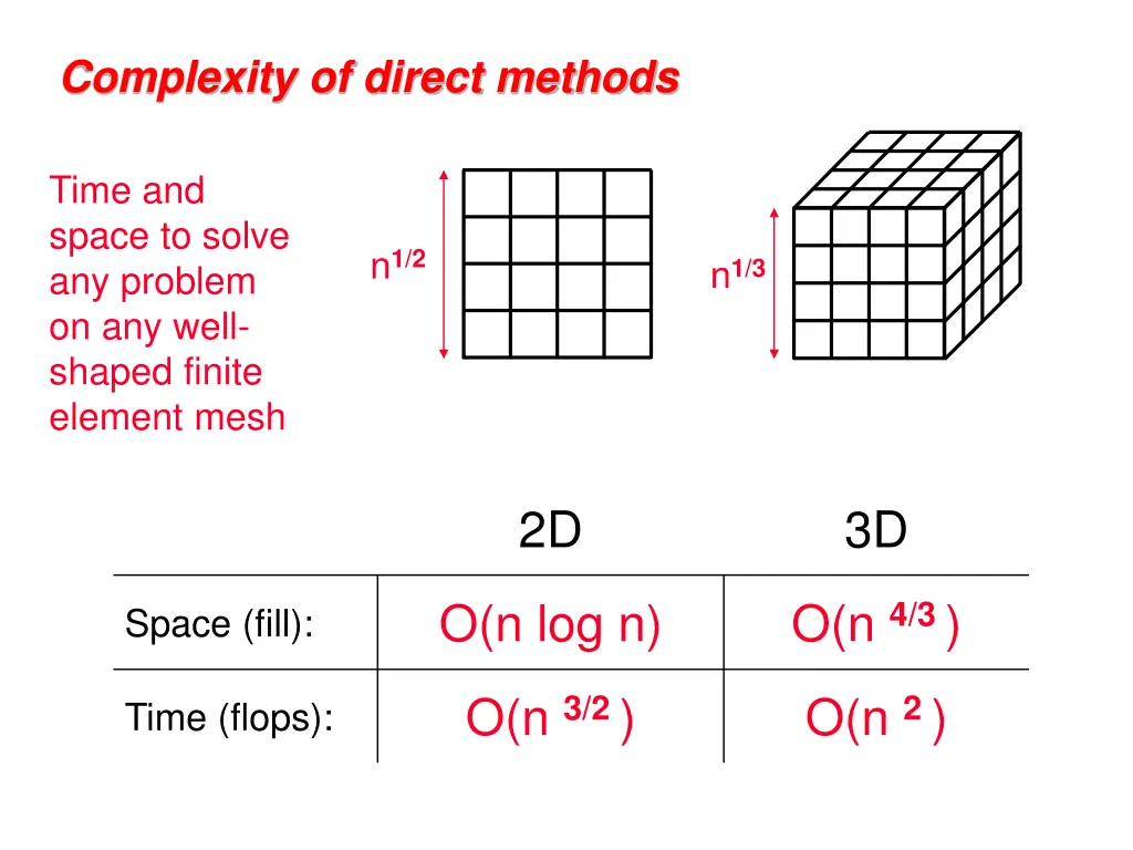
Complexity of direct methods Time and space to solve any problem on any well- shaped finite element mesh n1/2 n1/3 2D 3D O(n log n) O(n 4/3 ) Space (fill): O(n 3/2 ) O(n 2 ) Time (flops):

Complexity of linear solvers Time to solve model problem (Poisson s equation) on regular mesh n1/2 n1/3 2D O(n3 ) O(n1.5 ) 3D O(n3 ) O(n2 ) Dense Cholesky: Sparse Cholesky: CG, exact arithmetic: CG, no precond: CG, modified IC0: Support theory: Multigrid: O(n2 ) O(n1.5 ) O(n1.25 ) O~(n) O(n) O(n2 ) O(n1.33 ) O(n1.17 ) O~(n) O(n)

Hierarchy of matrix classes (all real) General nonsymmetric Diagonalizable Normal Symmetric indefinite Symmetric positive (semi)definite = Factor width n Factor width k . . . Factor width 4 Factor width 3 Symmetric diagonally dominant = Factor width 2 Generalized Laplacian = Symmetric diagonally dominant M-matrix Graph Laplacian

Definitions The Laplacian matrix of an n-vertex undirected graph G is the n-by-n symmetric matrix A with aij = -1 if i j and (i, j) is an edge of G aij = 0 if i j and (i, j) is not an edge of G aii = the number of edges incident on vertex i Theorem: The Laplacian matrix of G is symmetric, singular, and positive semidefinite. The multiplicity of 0 as an eigenvalue is equal to the number of connected components of G. A generalized Laplacian matrix (more accurately, a symmetric weakly diagonally dominant M-matrix) is an n-by-n symmetric matrix A with aij 0 if i j aii |aij| where the sum is over j i

Edge-vertex factorization of generalized Laplacians A generalized Laplacian matrix A can be factored as A = UUT, where U has: a row for each vertex a column for each edge, with two nonzeros of equal magnitude and opposite sign a column for each excess-weight vertex, with one nonzero vertices vertices A = U UT vertices edges (2 nzs/col) excess- weight vertices (1 nz/col) vertices

Support Graph Preconditioning CFIM: Complete factorization of incomplete matrix Define a preconditioner B for matrix A Explicitly compute the factorization B = LU Choose nonzero structure of B to make factoring cheap (using combinatorial tools from direct methods) Prove bounds on condition number using both algebraic and combinatorial tools +: New analytic tools, some new preconditioners +: Can use existing direct-methods software -: Current theory and techniques limited

Spanning Tree Preconditioner [Vaidya] G(A) G(B) A is generalized Laplacian (symmetric diagonally dominant with negative off-diagonal nzs) B is the gen Laplacian of a maximum-weight spanning tree for A (with diagonal modified to preserve row sums) Form B: costs O(n log n) or less time (graph algorithms for MST) Factorize B = RTR: costs O(n) space and O(n) time (sparse Cholesky) Apply B-1: costs O(n) time per iteration

Combinatorial analysis: cost of preconditioning G(A) G(B) A is generalized Laplacian (symmetric diagonally dominant with negative off-diagonal nzs) B is the gen Laplacian of a maximum-weight spanning tree for A (with diagonal modified to preserve row sums) Form B: costs O(n log n) time or less (graph algorithms for MST) Factorize B = RTR: costs O(n) space and O(n) time (sparse Cholesky) Apply B-1: costs O(n) time per iteration (two triangular solves)

Numerical analysis: quality of preconditioner G(A) G(B) support each edge of A by a path in B dilation(A edge) = length of supporting path in B congestion(B edge) = # of supported A edges p = max congestion, q = max dilation condition number (B-1A) bounded by p q (at most O(n2))

Spanning Tree Preconditioner [Vaidya] G(A) G(B) can improve congestion and dilation by adding a few strategically chosen edges to B cost of factor+solve is O(n1.75), or O(n1.2) if A is planar in experiments by Chen & Toledo, often better than drop-tolerance MIC for 2D problems, but not for 3D.

Numerical analysis: Support numbers Intuition from networks of electrical resistors: graph = circuit; edge = resistor; weight = 1/resistance = conductance How much must you amplify B to provide as much conductance as A? How big does t need to be for tB A to be positive semidefinite? What is the largest eigenvalue of B-1A ? The support of B for A is (A, B) = min { : xT(tB A)x 0 for all x and all t } If A and B are SPD then (A, B) = max{ : Ax = Bx} = max(A, B) Theorem: If A and B are SPD then (B-1A) = (A, B) (B, A)

Edge-vertex factorization of generalized Laplacians A generalized Laplacian matrix A can be factored as A = UUT, where U has: a row for each vertex a column for each edge, with two nonzeros of equal magnitude and opposite sign a column for each excess-weight vertex, with one nonzero vertices vertices A = U UT vertices edges (2 nzs/col) excess- weight vertices (1 nz/col) vertices

Algebraic Embedding Lemma [Boman/Hendrickson] Lemma: If V W=U, then (U UT, V VT) ||W||22 (with equality for some choice of W) Proof: take t ||W||22 = max(W WT) = max y 0 { yTW WTy / yTy } then yT (tI - W WT) y 0 for all y letting y = VTx gives xT (tV VT - U UT) x 0 for all x recall (A, B) = min{ : xT(tB A)x 0 for all x, all t } thus (U UT, V VT) ||W||22

-a2 -c2 -a2 -b2 -b2 [ ] [ ] a2 +b2-a2 -b2 -a2 a2 +c2 -c2 -b2 -c2 b2 +c2 a2 +b2-a2 -b2 -a2 a2 -b2 =VVT b2 B =UUT A -b-c[ ] U ] [ ab -a c ab -a c -b V

-a2 -c2 -a2 -b2 -b2 [ ] [ ] a2 +b2-a2 -b2 -a2 a2 +c2 -c2 -b2 -c2 b2 +c2 a2 +b2-a2 -b2 -a2 a2 -b2 =VVT [ b2 B =UUT A -b-c[ ] U ] [ ] ab -a c ab -a c 1-c/a 1 c/b/b B edges x = -b A edges V W

-a2 -c2 -a2 -b2 -b2 [ ] [ ] a2 +b2-a2 -b2 -a2 a2 +c2 -c2 -b2 -c2 b2 +c2 a2 +b2-a2 -b2 -a2 a2 -b2 =VVT [ b2 B =UUT A -b-c[ ] U ] [ ] ab -a c ab -a c 1-c/a 1 c/b/b B edges x = -b A edges V W (A, B) ||W||22 ||W|| x ||W||1 = (max row sum) x (max col sum) (max congestion) x (max dilation)

Extensions, remarks, open problems I Using another matrix norm inequality [Boman]: ||W||22 ||W||F 2= sum(wij2) = sum of (weighted) dilations, and [Alon, Karp, Peleg, West] construct spanning trees with average weighted dilation exp(O((log n loglog n)1/2)) = o(n ). This gives condition number O(n1+ ) and solution time O(n1.5+ ), compared to Vaidya s O(n1.75) with augmented MST. Is there a graph construction that minimizes ||W||22directly? [Spielman, Teng]: complicated recursive partitioning construction with solution time O(n1+ ) for all generalized Laplacians! (Uses yet another matrix norm inequality.)

Extensions, remarks, open problems II Support theory methods for more general matrices? [Boman, Chen, Hendrickson, Toledo]: different matroid for all symmetric diagonally dominant matrices (= factor width 2). Matrices of bounded factor width? Factor width 3? All SPD matrices? Is there a version that s useful in practice? Especially for non-geometric graph Laplacians? [Koutis, Miller, Peng 2010] simplifies Spielman/Teng a lot. [Kelner et al. 2013] : random Kaczmarz projections in the dual space even simpler, good O() theorems, but not yet fast enough in practice. Lots of current work.

Support-graph analysis of modified incomplete Cholesky -1 -1 -1 -1 -1 -1 -1 -1 -1 -1 -1 -1 -1 -1 .5 .5 .5 -1 -1 -1 -1 -1 -1 B A -1 -1 -1 -1 -1 -1 -1 -1 .5 .5 .5 -1 -1 -1 -1 -1 -1 -1 -1 -1 -1 -1 -1 -1 -1 .5 .5 .5 -1 -1 -1 -1 -1 -1 A = 2D model Poisson problem B = MIC preconditioner for A B has positive (dotted) edges that cancel fill B has same row sums as A Strategy: Use the negative edges of B to support both the negative edges of A and the positive edges of B.

Supporting positive edges of B Every dotted (positive) edge in B is supported by two paths in B Each solid edge of B supports one or two dotted edges Tune fractions to support each dotted edge exactly 1/(2 n 2) of each solid edge is left over to support an edge of A

Analysis of MIC: Summary Each edge of A is supported by the leftover 1/(2 n 2) fraction of the same edge of B. Therefore (A, B) 2 n 2 Easy to show (B, A) 1 For this 2D model problem, condition number is O(n1/2) Similar argument in 3D gives condition number O(n1/3) or O(n2/3) (depending on boundary conditions)