Measurements of Central Tendency in Statistics
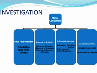
Explore the concept of central tendency in statistics, covering arithmetic mean, median, mode, geometric mean, and harmonic mean. Learn how to calculate these measures in different types of data series. Understand the relationships between mean, median, and mode for effective data analysis.

Download Presentation

Please find below an Image/Link to download the presentation.
The content on the website is provided AS IS for your information and personal use only. It may not be sold, licensed, or shared on other websites without obtaining consent from the author. If you encounter any issues during the download, it is possible that the publisher has removed the file from their server.
You are allowed to download the files provided on this website for personal or commercial use, subject to the condition that they are used lawfully. All files are the property of their respective owners.
The content on the website is provided AS IS for your information and personal use only. It may not be sold, licensed, or shared on other websites without obtaining consent from the author.
E N D
Presentation Transcript
Measurements of central tendency
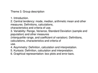
Introduction Arithmetic mean Median Mode Geometric mean Harmonic mean Relationship b/w mean, median & mode
Arithmetic mean Calculation of arithmetic mean in the following ways: i) In a series of individual observations ii) In a discrete series iii) In a continuous series
i) In a series of individual observations Equation: X = ? ? = AM = Sum of all the observations = number of observations x X n For example: calculate the arithmetic mean of following observations x = 2, 4, 6, 8, 10, 20, 12, 20
ii) In a series of discrete observations X = ?? Equation: ? x = AM fX = sum of values of variables and corresponding frequencies f = sum of frequencies For observations example: calculate the arithmetic mean of following x 2 4 6 10 12 f 3 5 2 2 4
iii) In a series of continuous series X = ?? The histogram can be constructed in two ways depending up class- interval: x = AM fm = sum of values of mid-point and corresponding frequencies f = sum of frequencies Equation: ? a) For distributions that have equal class intervals b) For distributions that have unequal class intervals CI 10-20 20-30 30-40 For example: calculate the arithmetic mean of following observations 40-50 50-60 60-70 f 3 5 2 2 4 4
Median The median is usually defined as that value which divides a distribution so that an equal number of items occur on either side of it. The histogram can be constructed in two ways depending up class- interval: 50% of the observations will be smaller than the median, if the number of value is odd, the median will be middle value. a) For distributions that have equal class intervals b) For distributions that have unequal class intervals The data should be arranged in ascending or descending order
Median The histogram can be constructed in two ways depending up class- interval: M =?+1 i) Calculation of median in a series of individual observations a) Arrange the data in ascending or descending order b) Median is calculated by finding the value of n+1/2th item 2 a) For distributions that have equal class intervals b) For distributions that have unequal class intervals For example: calculate the median of following observations x = 2, 4, 6, 8, 10, 20, 12, 20, 2, 13, 45, 5, 16, 14, 11
Median The histogram can be constructed in two ways depending up class- interval: b) Find out the CF c) Median: the value of n+1/2th item d) It can be found by first locating the cumulative frequency which is equal to n+1/2 or the next higher to this and then determine the value corresponding to it. It will be M i) Calculation of median in a discrete series a) Arrange the data in ascending or descending order a) For distributions that have equal class intervals b) For distributions that have unequal class intervals x 2 14 6 For example: calculate the median of following observations 10 22 12 16 f 3 5 2 2 4 5 8
i) Calculation of median in a discrete series cf cf X F F Solution: M = size of ?+1 2 3 3 2 3 2th item M = 29+1 6 2 5 14 5 2 = 15th item (more close to 15th item) M = 22 10 2 7 6 2 12 5 12 10 2 14 5 17 22 4 16 8 25 12 5 22 4 29 16 8
Median The histogram can be constructed in two ways depending up class- interval: ii) Calculation of median in a continuous series ? 2 ?? ? x i L = lower limit of the medianclass M = ? + cf = cumulative frequency of the class preceding the median class F = frequency of the median class i = class interval a) For distributions that have equal class intervals b) For distributions that have unequal class intervals CI 2 14 6 CI 10-20 20-30 30-40 For example: calculate the median of following observations 10 40-50 22 12 50-60 16 60-70 f f 3 3 5 5 2 2 2 4 2 5 4 8 4
ii) Calculation of median in continuous series cf cf CI F Solution: M = size of ? 3 10-20 3 2 th item M = 20 8 20-30 5 2 = 10th item (median lies in the class = 30-40) L = 30, cf = 8, i= 10, f= 2 10 30-40 2 12 40-50 2 x 10 = ? M = 30 +10 8 16 50-60 4 2 20 60-70 4
Exercise Exercise no. no. 10 Calculate the median in following observation 10 Calculate the median in following observation CI 10-20 2 20-30 3 30-40 4 40-50 2 50-60 4 60-70 5 70-80 8 F Exercise no. 11 Calculate the median in following observation Exercise no. 11 Calculate the median in following observation CI F 10-20 2 20-30 3 30-60 12 60-80 10 80-90 4 90-100 8
Exercise no. 11 Calculate the median in following observation Exercise no. 11 Calculate the median in following observation CI F CF 10-20 2 2 20-30 30-40 3 4 5 9 40-50 4 13 50-60 4 17 60-70 5 22 70-80 5 27 80-90 4 31 90-100 8 39
Graphic location of median Median can be located graphically by applying any one of the following methods: i) Draw only one ogive curve by less than & more than method ii) Draw two ogives curve one by less than & other by more than method For example: Determine the value of median graphically CI 10-20 20-30 30-40 40-50 50-60 60-70 f 3 5 2 2 4 4
Graphic location of median cf cf CI f Less than ogive More than ogive cf Cf Variable Variable 10-20 3 3 20 10 3 20 20-30 5 8 30 20 8 10 16 12 30-40 2 10 40 30 50 40 12 10 40-50 2 12 60 50 16 8 50-60 4 16 70 60 20 3 60-70 4 20 70 0
Mode The mode is another measure of central tendency Mode is the most typical value of a distribution because it is repeated the highest number of items in the series The mode of a distribution is the value at the point around which the items tend to be most heavily concentrated Two types a) Unimodal b) Bimodal or multimodal
Mode The mode is another measure of central tendency Mode is the most typical value of a distribution because it is repeated the highest number of items in the series The mode of a distribution is the value at the point around which the items tend to be most heavily concentrated Two types a) Unimodal b) Bimodal or multimodal For example: x = 8,9,10,2,5,8,16,18,14,7 x = 8,9,10,2,5,8,16,18,14,10 x = 6,7,8,9,10,11,12,15,4,5,20
Mode in symmetrical and skewed distributions In perfectly symmetrical distribution, there is only one mode, the three measures of central tendency the mode, median & mean coincide with the highest point There are three distributions of central tendency a) Symmetrical distribution (Mo=Me=Mean) b) Positively skewed distribution (Mo>Me>Mean) c) Negatively skewed distribution
Mode in symmetrical and skewed distributions a) Symmetrical distribution In such there is only one mode, the three measures of central tendency the mode, median & mean coincide with the highest point b) Positively skewed distribution The mode is at the highest point and the median lies to the right of this point, but mean falls to the right of the median c) Negatively skewed distribution The mode will have the largest value, the median lies to the left of the mode and the mean falls to the left of the median
Mode in symmetrical and skewed distributions X = 2,4,8,10,8,6,7,9,12
Mode In continuous series, the modal class should be ascertained first which defined as the class having maximum frequency b) Calculation of mode in a continuous series is 1 + 2x i 1 Mode = ? + Equation: L = Lower limit of the modal class 1 = Difference b/w the frequency of the modal class and the frequency of the preceding class (ignore sign) 2 = Difference b/w the frequency of the modal class and the frequency of the succeeding class (ignore signs) i = class interval
b) Calculation of mode in a continuous series For example: Calculate the mode for following distribution CI 10-20 20-30 30-40 40-50 50-60 60-70 Solution: Mode lies in the class = 20 30 L = 20, 1= (5 - 3) = 2, 1 1 + 2x i 2 = (5 2) = 3, i = 10 2 +3x 10 = ? f 3 5 2 2 4 4 Mode = ? + 2 = 20 +
c) Graphic location of mode For example: Calculate the mode for following distribution CI 10-20 20-30 30-40 40-50 50-60 60-70 f 3 5 2 2 4 4 6 5 4 Frequency 3 2 1 0 10-20 20-30 30-40 Class Interval 40-50 50-60 60-70
Relationship between Mean, Median and Mode Equation: Mean - Mode = 3(Mean Median) Mode = 3 Median 2 Mean For exp: Calculate the mean if the mode is 11 and median is 14. Mean = 15.5


 In a series of individual observations")
 In a series of discrete observations")
 In a series of continuous series")


 Calculation of median in a discrete series")

 Calculation of median in continuous series")


 Calculation of mode in a continuous series")
 Graphic location of mode")