Measures of Central Tendency and Data Description

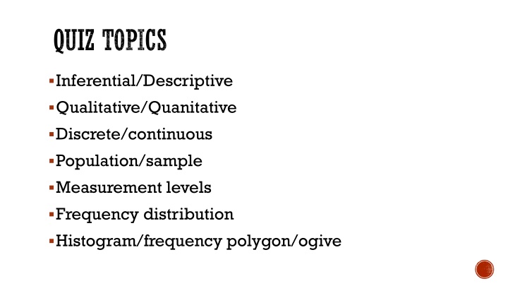
QUIZ TOPICS Inferential/Descriptive Qualitative/Quanitative Discrete/continuous Population/sample Measurement levels Frequency distribution Histogram/frequency polygon/ogive

DO NOW What do you remember about mean, median, and mode?

HOW DO WE MEASURE DATA? Center, spread, position

WHAT DO WE MEAN WHEN WE SAY AVERAGE ? The average American man is 5 9 . The average woman is 5 3.6 . The average American is sick in bed 7 days a year missing 5 days of work. On an average day, 24 million people receive animal bites. By his or her 70thbirthday, the average American will have eaten 14 steers, 1050 chickens, 3.5 lambs, and 25.2 hogs.

HOW WE DESCRIBE DATA Knowing the average is not enough to describe the data Also need to know how the data is spread around the average Need to be able to find where a specific data value falls within the data set or its relative position in comparison with the other data values.

HOW WE DESCRIBE DATA Measures of central tendency mean, median, mode, midrange Measures of variation range, variance, standard deviation Measures of position percentiles, deciles, quartiles Exploratory data analysis box plots, five-number summaries

MEASURES OF CENTRAL TENDENCY First we must distinguish if we are taking the average of a sample or of an entire population. Statistic a characteristic or measures obtained by using the data values from a sample. (***Use Roman letters) Parameter a characteristic of measure obtained by using all the data values from a specific population. (***Use Greek letters) General Rounding Rule: Rounding should not be done until the final answer is calculated; otherwise, there could be multiple rounding errors.

MEAN Arithmetic average Add values and divide by number of values (you re used to this). Should be rounded to one more decimal place than occurs in the raw data. ( = mew)

MEAN Usually, finding the mean is easy, but grouped frequencies are a little different Procedure: 1. Make a table as shown. Formula for mean of grouped frequency A B C D Class Frequency f Midpoint Xm f Xm 2. Find the midpoints of each class and place them in Column C. 3. Multiply the frequency by the midpoint for each class, and place the product in Column D. 4. Find the sum of Column D. 5. Divide the sum obtained in Column D by the sum of the frequencies obtained in Column B.

EXAMPLE FOR MEAN OF GROUPED FREQUENCY Find the mean of the following data set: Class Limits Class Boundaries 23.5-30.5 30.5-37.5 37.5-44.5 44.5-51.5 51.5-58.5 58.5-65.5 Tally Frequency 24-30 31-37 38-44 45-51 52-58 59-65 I I I I I I I I I I I I I I I I I I I I I I I I I 3 1 5 9 6 1

WEIGHTED MEAN Used when not all values are equally represented. Procedure: Multiply each value by its corresponding weight Divide the sum of the products by the sum of the weights

GRADE POINT AVERAGE A student received an A in English Composition I (3 credits), a C in Intro to Psych (3 credits), a B in Bio I (4 credits), and a D in Phys Ed (2 credits). Assuming A = 4 grade points, B = 3 grade points, C = 2 grade points, D = 1 grade point, and F = 0 grade points, find the student s overall GPA. Course Eng Comp Intro Psych Bio I Phys Ed Credits (w) 3 3 4 2 Grade (x) A (4 pts) C (2 pts) B (3 pts) D (1 pt)

MEDIAN Midpoint of the data array. Denoted MD. Procedure: Arrange data in order (all data! No matter how many times a number comes up.) Select middle point

MODE The value that occurs most often in the data set. Unimodal data set has one mode Bimodal data set has two modes Multimodal data set has more than 2 modes No mode when no data value occurs more than once Modal Class Class with the highest frequency in a grouped frequency distribution

MIDRANGE Rough estimate of the middle Add the lowest and highest values in the data set, and divide by 2. Very rough estimate of the average and can be affected by extreme high or low values. Denoted MR

DISTRIBUTION SHAPES

DO NOW Find the mean for Brand A and Brand B. Do you think the mean is accurate representation of both sets of data? Brand A Brand B 10 35 60 45 50 30 30 35 40 40 20 25

MEASURES OF VARIATION The data shows how long two brands of outdoor paint last in months. -The mean for Brand A is 35 months. -The mean for Brand B is 35 months. Brand A Brand B 10 35 60 45 50 30 30 35 Even though the means are equal, the spread or variation is quite different. Brand B is more consistent, less variable. Brand A is more spread, less consistent. 40 40 20 25

RANGE Highest value minus lowest value Brand A Brand B Denoted R 10 35 60 45 Brand A R = 60 10 = 50 months 50 30 30 35 Brand B R = 45 25 = 20 months 40 40 20 25

Variance The average of the squares of the distance each value is from the mean. Standard Deviation The square root of the variance Denoted (sigma) Denoted 2 (sigma squared) Rounding rule for Standard Deviation same as the mean; the final answer should be rounded to one more decimal place than that of the original data.

Population Variance ( 2) Sample Variance (s2) Shortcut Formula for Sample Standard Deviation Standard Deviation ( ) Standard Deviation (s)

VARIANCE AND STANDARD DEVIATION FOR GROUPED DATA Procedure: 1. Make a table as shown and find the midpoint of each class. A B C D E Class Frequency Midpoint f Xm f X2m 2. Multiply the frequency by the midpoint for each class, and place the products in column D. 3. Multiply the frequency by the square of the midpoint and place the product in column E. 4. Find the sums of columns B, D, and E. 5. Substitute in the formula and solve for s2 to get the variance. 6. Take the square root to get the standard deviation.

EXAMPLE FOR VARIANCE OF GROUPED FREQUENCY Find the mean of the following data set: Class Limits Class Tally Frequency Boundaries 23.5-30.5 30.5-37.5 37.5-44.5 44.5-51.5 51.5-58.5 58.5-65.5 24-30 31-37 38-44 45-51 52-58 59-65 I I I I I I I I I I I I I I I I I I I I I I I I I 3 1 5 9 6 1

DO NOW Find the mean, median, and mode for the following data set: 2, 6, 3, 9, 5, 6, 2, 6

COEFFICIENT OF VARIATION Allows you to compare standard deviations when the units are different such as comparing the number of sales per salesperson over a 3-month period and the commissions made by these salespeople. Standard deviation divided by the mean, expressed as a percentage. Denoted by CVar

RANGE RULE OF THUMB A rough estimate of standard deviation is s range 4 ***Only as approximation Should be used when the distribution of data values is unimodal and roughly symmetric. Can be used to estimate the largest and smallest data values of a data set. Approximately 2 standard deviations away from the mean

CHEBYSHEVS THEOREM We know that the larger the variance or standard deviation, the more the data values are dispersed. Chebyshev s Theorem specifies the proportions of the spread in terms of the standard deviation. Chebyshev s Theorem: The proportion of values from a data set that will fall within k standard deviations of the mean will be at least 1 is not necessarily an integer). 1 ?2, where k is a number greater than 1 (k This theorem can be applied to any distribution, no matter the shape. For example, this theorem states that at least (75%) of the data values will fall within 2 standard deviations of the mean of the data set (when k = 2).

CHEBYSHEVS THEOREM EXAMPLES Example 1 The mean price of houses in a certain neighborhood is $50,000, and the standard deviation is $10,000. Find the price range for which at least 75% of the houses will sell. Example 2 A survey of local companies found that the mean amount of travel allowance for executives was $0.25 per mile. The standard deviation was $0.02. Using Chebyshev s Theorem, find the minimum percentage of the data values that will fall between $0.20 and $0.30.

EMPIRICAL RULE Chebyshev s Theorem applies to ANY distribution, regardless of shape. However, when a distribution is bell-shaped (or what is called normal), the following statements, which make up the empirical rule are true: Approximately 68% of the data values will fall within 1 standard deviation of the mean. Approximately 95% of the data values will fall within 2 standard deviation of the mean. Approximately 99.7% of the data values will fall within 3 standard deviation of the mean.

EMPIRICAL RULE EXAMPLE Suppose that the scores on a national achievement exam have a mean of 480 and a standard deviation of 90. If these scores are normally distributed, then Approximately 68% will fall between ______ and _______, Approximately 95% will fall between ______ and _______, And approximately 99.7% will fall between ______ and ______.

SKILLS CHECK BLOOD PRESSURE Apply Chebyshev s Theorem to the systolic blood pressure of normotensive men. At least how many of the men in the study fall within 1 standard deviation of the mean? At least how many of those men in the study fall within 2 standard deviations of the mean? Give the ranges for the diastolic blood pressure (normotensive and hypertensive) of older women. Assume normal distribution. Do the normotensive, male, systolic blood pressure ranges overlap with the hypertensive, male, systolic blood pressure ranges? Assume normal distribution. 1. Normotensive Men (n=1200) 55 10 Hypertensive Men (n=1100) 60 10 Women (n=1400) 55 10 Women (n=1300) 64 10 Age Blood Pressure (mm Hg) 2. 3. Systolic Diastoli c 123 9 78 7 121 11 76 7 153 17 91 10 156 20 88 10 4.

MEASURES OF POSITION Objective: Identify the position of a data value in a data set, using various measures of position, such as percentiles, deciles, and quartiles.

STANDARD SCORES (Z SCORES) Suppose you got a 90 on a music test, and a 45 on an English test. Direct comparison of raw scores is impossible, since the exams might not be equivalent in terms of the number of questions, value of each question, and so on. However, a comparison of a relative standard similar to both can be made. This comparison uses the mean and standard deviation and is called a standard score, or z score. A z score tells how many standard deviations a data value is above or below the mean for a specific distribution of values. Z>0: above the mean Z=0: equal to the mean Z<0: below the mean

STANDARD SCORES (Z SCORES) A z score or standard score for a value is obtained by subtracting the mean from the value and dividing that result by the standard deviation. Denoted z Represents the number of standard deviations a data value falls above or below the mean Samples Populations

STANDARD SCORES (Z SCORES) Example A student scored 65 on a calculus test that had a mean of 50 and standard deviation of 10; she scored 30 on a history test with a mean of 25 and standard deviation of 5. Compare her relative positions on the two tests. When all data for a variable are transformed into z scores, the resulting distribution will have a mean of 0 and a standard deviation of 1. A z score, then, is actually the number of standard deviations each value is from the mean for a specific distribution. How many standard deviations was the calculus score from the mean? Above or below?

PERCENTILES Divide the data set into 100 equal parts. For standardized tests, when they tell you that you scored in the 77th percentile, that means you scored higher than 77% of the people who took the test. ***Different from percents scoring a 72% and scoring in the 72nd percentile are two different things. Percent tells you how many you got correct. Percentile compares you to others taking the test.

PERCENTILES The percentile corresponding to a given value X is computed by using the following formula: Finding the value that corresponds to a given percentile uses the following formula: c = value at given percentile n = total number of values P = percentile B = number of values BELOW given value E = number of values EQUAL to given value n = total number of values When c is not whole, round up to nearest whole number. When c is whole, use value halfway between c and (c+1) values

PERCENTILES Example 1 A teacher gives a 20-point test to 10 students. The scores are shown here. Find the percentile rank of a score of 12. 18, 15, 12, 6, 8, 2, 3, 5, 20, 10 Example 2 Using these same scores, find the value corresponding to the 25th percentile.

PERCENTILES Deciles Quartiles Divide distribution into ten groups Divide distribution into four groups Denoted D1, D2, etc. Separated by Q1, Q2, Q3 Q1 = 25th percentile Q2 = median (50th percentile) Q3 = 75th percentile Interquartile Range (IQR): Q3 Q1

OUTLIERS An extremely high or an extremely low data value when compared with the rest of the data values. Can strongly affect the mean and standard deviation of a variable, as we have seen before. To identify outliers: Arrange data in order and find Q1 and Q3. Find the IQR Multiply IQR by 1.5 Subtract value obtained from Q1, and add the value to Q3. Check the data set for any data that is smaller than Q1 1.5(IQR) or larger than Q3 + 1.5(IQR)

OUTLIERS Example Check the following data set for outliers 5, 6, 12, 13, 15, 18, 22, 50

SKILLS CHECK In an attempt to determine necessary dosages of a new drug (HDL) used to control sepsis, assume you administer varying amounts of HDL to 40 mice. You create four groups and label them low dosage, moderate dosage, large dosage, and very large dosage. The dosages also vary within each group. After the mice are injected with the HDL and the sepsis bacteria, the time until the onset of sepsis is recorded. Your job as a statistician is to effectively communicate the results of the study. Which measures of position could be used to help describe the data results? 1. If 40% of the mice in the top quartile survived after the injection, how many mice would that be? 2. What info can be given from using percentiles? 3. What info can be given using quartiles? 4. What info can be given from using standard scores? 5.

EXPLORATORY DATA ANALYSIS The purpose of Exploratory Data Analysis is to examine data to find out what information can be discovered about the data such as the center and the spread. Data is organized using stem and leaf plots Central tendency = median Measure of variation = IQR (interquartile range) Represented graphically using a boxplot

THE FIVE-NUMBER SUMMARY AND BOXPLOTS A boxplot graphically represents data using the following specific values: Minimum Q1 Median Q3 Maximum These values are called a five-number summary of the data set.

PROCEDURE FOR CONSTRUCTING BOXPLOTS 1. Find the five-number summary for the data values Draw a horizontal axis with a scale such that it includes the maximum and minimum data values. 2. Draw a box whose vertical sides go through Q1 and Q3, and draw a vertical line through the median. 3. Draw a line from the minimum data value to the left side of the box and a line from the maximum data value to the right side of the box. 4.

INFORMATION OBTAINED FROM BOXPLOTS Median If the median is near the center of the box, the distribution is approximately symmetric. If the median falls to the left of the center of the box, the distribution is positively (right) skewed. If the median falls to the right of the center of the box, the distribution is negatively (left) skewed. Lines If the lines are about the same length, the distribution is approximately symmetric. If the right line is longer than the left line, the distribution is positively (right) skewed. If the left line is longer than the right line, the distribution is negatively (left) skewed.

BOXPLOTS Example 1 The number of meteorites found in 10 states of the United States is 89, 47, 164, 296, 30, 215, 138, 78, 48, 39. Construct a boxplot for the data. Example 2 A dietician is interested in comparing the sodium content of real cheese with the sodium content of cheese substitute. The data for two random samples are shown. Compare the distributions using boxplots. Real Cheese 420 240 Cheese Substitute 180 260 310 220 45 180 40 90 270 130 250 340 290 310

RESISTANT AND NONRESISTANT STATISTICS Resistant Statistics less affected by outliers Median IQR Nonresistant Statistics more affected by outliers Mean Standard deviation Sometimes when a distribution is skewed or contains outliers, the median and IQR may more accurately summarize the data than the mean and standard deviation, since the mean and standard deviation are more affected in this case.

TRADITIONAL VS. EDA TECHNIQUES Traditional Exploratory Data Analysis Stem and Leaf Plot Frequency Distribution Histogram Mean Standard Deviation Boxplot Median Interquartile Range