Methods for Dummies 2013: Spatial Normalisation and Registration Techniques
This content delves into the methods described in the book "Methods for Dummies 2013" by Elin Rees and Peter McColgan. It covers various processes such as pre-processing, spatial normalisation, segmentation, modulation, smoothing, statistical analysis, GLM, group comparisons, correlations, longitudinal fluids, interpretation, and addressing issues like multiple comparisons. Additionally, it discusses the use of Statistical Parametric Mapping software for unbiased techniques, pre-processing alignment, parametric statistics, and generating statistical parametric maps that showcase differences between groups. The iterative tissue classification, normalisation, and bias correction process is detailed, involving segmentation, affine registration, normalisation, and bias correction steps. The Diffeomorphic Anatomical Registration technique using Exponentiated Lie algebra registration is explained, focusing on GM segmentation registration to a standard space. Furthermore, spatial normalisation, modulation of segmentations, and rescaling of intensities are explored in detail.

Download Presentation

Please find below an Image/Link to download the presentation.
The content on the website is provided AS IS for your information and personal use only. It may not be sold, licensed, or shared on other websites without obtaining consent from the author.If you encounter any issues during the download, it is possible that the publisher has removed the file from their server.
You are allowed to download the files provided on this website for personal or commercial use, subject to the condition that they are used lawfully. All files are the property of their respective owners.
The content on the website is provided AS IS for your information and personal use only. It may not be sold, licensed, or shared on other websites without obtaining consent from the author.
E N D
Presentation Transcript
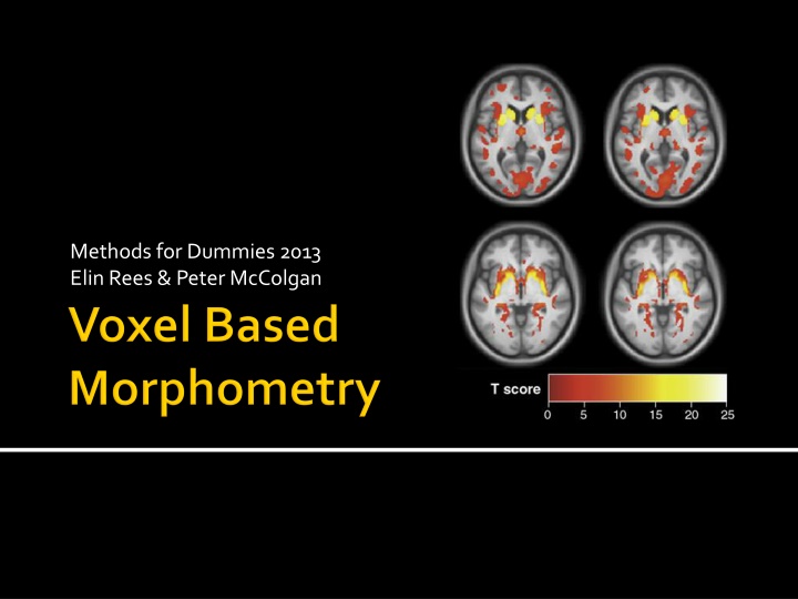
Methods for Dummies 2013 ElinRees & Peter McColgan
General idea Pre-Processing Spatial normalisation Segmentation Modulation Smoothing Statistical analysis GLM Group comparisons Correlations Longitudinal fluids Interpretation Issues Multiple comparisons Controlling for TIV Global or local change Interpreting results Summary
Uses Statistical Parametric Mapping software Unbiased technique Pre-processing to align all images Parametric statistics at each point within the image Mass-univariate Statistical parametric map showing e.g. differences between groups regions where there is a significant correlation with a clinical measure
= iterative tissue classification + normalisation + bias correction Segmentation: Models the intensity distributions by a mixture of Gaussians, but using tissue probability map (TPM) to weight the classification TPM = priors of where to expect certain tissue types Affine registration of scan to TPM Normalisation: The transform used to align the image to the TPM used to normalise the scan to standard (TPM) space parameters calculated but not applied Corrects for global brain shape differences Bias correction: Spatially smoothes the intensity variability, which is worse at higher field strengths
= Diffeomorphic Anatomical Registration using Exponentiated Lie algebra registration Registration of GM segmentations to a standard space 1) Applies affine parameters into TPM space 2) Additional non-linear warp to study specific space Study-specific grey matter template Constructs a flow field so one image can slowly flow into another Allows for more precise inter-subject alignment Involves prior knowledge e.g. stretches, scales, shifts and warps
Spatial normalisation removes differences between scans Modulation of segmentations puts this information back Rescaling the intensities dependent on the amount of expansion/contraction - if not much change needed, not much intensity change E.g. Native = Unmodulated warped = 1 Modulated = 2/3 = lower in the middle where imaged stretched but total is preserved. 1 1 1/3 1 1 1/3 1 2/3
Gets rid of roughness and noise to produce data in a more normal distribution Removes some registration errors Kernel defined in terms of FWHM (full width at half maximum) of filter 7-14mm kernel Analysis is most sensitive to effects that match the shape and size of the kernel Match Filter Theorem Kernel takes weighted average of the surrounding intensities Smaller kernels mean results can be localised to a more precise region Less smoothing needed if DARTEL used In an ideal world this would not be needed
Voxel-wise (mass-univariate) independent statistical tests for every single voxel Group comparison: Regions of difference between groups Correlation: Region of association with test score
Test group differences in e.g. grey matter BUT which covariates e.g. age, gender etc.? which search volume? what threshold? correction for multiple comparisons? Ridgeway et al. 2008: Ten simple rules for reporting voxel-based morphometry studies Multiple methodological options available Decisions must be clearly described Henley et al. 2009: Pitfalls in the Use of Voxel-Based Morphometry as a Biomarker: Examples from Huntington Disease
GLM Y = X + Intensity for each voxel (V) is a function that models the different things that account for differences between scans: V = 1(Subject A) + 2(Subject B) + 3(covariates) + 4(global volume) + + V = 1(test score) + 2(age) + 3(gender) + 4(global volume) + +
SPM Mass univariate independent statistical tests for every voxel ~ 1000,000 Regions of significantly less grey matter intensity between subjects and controls Regions showing a significant correlation with test score or clinical measure
Multiple Comparisons Introducing false positives when dealing with one than one statistical comparison One t-test with p < .05 a 5% chance of (at least) one false positive 3 t-tests, all at p < .05 All have 5% chance of a false positive So actually you have 3 x 5% chance of a false positive = 15% chance of introducing a false positive
How big is the problem? In VBM, depending on your resolution 1000000 voxels 1000000 statistical tests do the maths at p < .05! 50000 false positives So what to do? Bonferroni Correction Random Field Theory/ Family-wise error False Discovery Rate Small Volume Correction
Bonferroni-Correction (controls false positives at individual voxel level): divide desired p value by number of comparisons .05/1000000 = p < 0.00000005 at every single voxel Not a brilliant solution (false negatives) Added problem of spatial correlation data from one voxel will tend to be similar to data from nearby voxels
Family Wise Error (FWE) Probability that one or more of the significance tests results is a false positive within the volume of interest SPM uses Gaussian Random Field Theory (GRFT) GRFT finds right threshold for a smooth statistical map which gives the required FWE. It controls the number of false positive regions rather than voxels Allows multiple non-independent tests
False Discovery Rate Controls the expected proportion of false positives among suprathreshold voxels only Using FDR, q<0.05: we expect 5% of the voxels for each SPM to be false positives (1,000 voxels) Bad: less stringent than FWE so more false positives Good: fewer false negatives (i.e. more true positives) More lenient may be better for smaller studies
Small Volume Correction Hypothesis driven and ideally based on previous work Place regions of interest over particular structures Reduces the number of comparisons Increases the chance of identifying significant voxels in a ROI
Controlling for total intracranial volume (TIV) Uniformly bigger brains may have uniformly more GM/ WM brain A brain B brain A brain B Differences without accounting for TIV differences after TIV has been covaried out (Differences uniformally distributed with hardly any impact at local level)
Global or local change With TIV: greater volume in A relative to B only in the thin area on the right-hand side Without TIV: greater volume in B relative to A except in the thin area on the right-hand side Including total GM or WM volume as a covariate adjusts for global atrophy and looks for regionally-specific changes
Longitudinal Analysis: Fluid Registration Baseline and follow-up image are registered together non-linearly Voxels at follow-up are warped to voxels at baseline Represented visually as a voxel compression map showing regions of contraction and expansion contracting expanding
Small volume structures: Hippocampus and Caudate, issues with normalisation and alignment VBM in degenerative brain disease: normalisation, segementation and smoothing of atrophied scans
Disadvantages Advantages Data collection constraints (exactly the same way) Fully automated: quick and not susceptible to human error and inconsistencies Statistical challenges Results may be flawed by preprocessing steps Unbiased and objective Not based on regions of interests; more exploratory Underlying cause of difference unknown Interpretation of data- what are these changes when they are not volumetric? Picks up on differences/ changes at a global and local scale Has highlighted structural differences and changes between groups of people as well as over time


")


")


")