Methods for Finding Roots of Non-Linear Equations Recap
Explore various methods such as graphical, bracketing, open methods, special methods for polynomials, and hybrid methods for finding roots of non-linear equations, along with a detailed explanation of the Muller method. Learn how to fit a quadratic polynomial through three points to approximate a function and understand the concept of divided differences. Discover properties of divided differences and how they can be utilized in solving equations.

Download Presentation

Please find below an Image/Link to download the presentation.
The content on the website is provided AS IS for your information and personal use only. It may not be sold, licensed, or shared on other websites without obtaining consent from the author. If you encounter any issues during the download, it is possible that the publisher has removed the file from their server.
You are allowed to download the files provided on this website for personal or commercial use, subject to the condition that they are used lawfully. All files are the property of their respective owners.
The content on the website is provided AS IS for your information and personal use only. It may not be sold, licensed, or shared on other websites without obtaining consent from the author.
E N D
Presentation Transcript
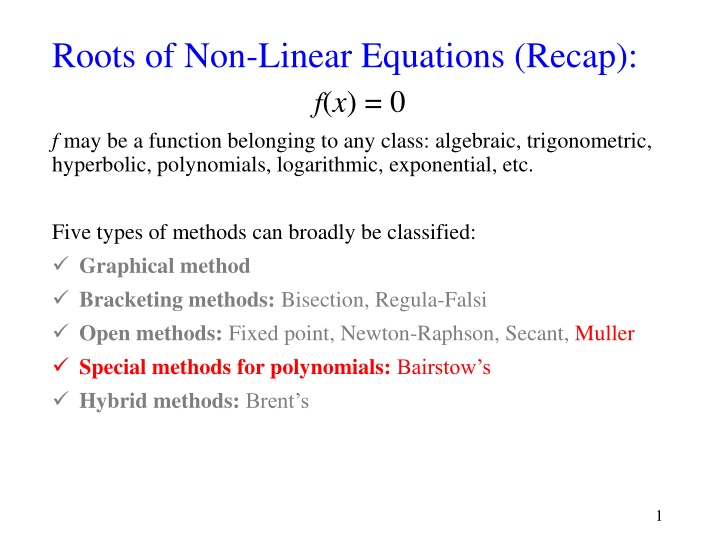
Roots of Non-Linear Equations (Recap): f(x) = 0 f may be a function belonging to any class: algebraic, trigonometric, hyperbolic, polynomials, logarithmic, exponential, etc. Five types of methods can broadly be classified: Graphical method Bracketing methods: Bisection, Regula-Falsi Open methods: Fixed point, Newton-Raphson, Secant, Muller Special methods for polynomials: Bairstow s Hybrid methods: Brent s 1
Open Methods: Muller Principle: fit a quadratic polynomial through three points to approximate the function. Problem: f(x) = 0, find a root x = such that f( ) = 0 f(x0) f(x1) f(x2) x2 x0 x1 y = f(x) x3 2
Open Methods: Muller Initialize: choose three points x0, x1, x2 and evaluate f(x0), f(x1), f(x2). Denote f(xk) = fk Fit a quadratic polynomial through three points xk, xk-1, xk-2 as: p(x) = a(x - xk)2 + b(x - xk) + c Equations: p(xk) = fk = c p(xk-1) = fk-1= a(xk-1- xk)2 + b(xk-1- xk) + fk p(xk-2) = fk-2 = a(xk-2- xk)2 + b(xk-2- xk) + fk Define Divided Differences: 1st Divided Difference:? ??,?? 1 =? ?? ? ?? 1 ?? ?? 1 2nd Divided Difference: ? ??,?? 1,?? 2 =? ??,?? 1 ? ?? 1,?? 2 ?? ?? 2 3
Open Methods: Muller p(xk) = fk = c p(xk-1) = fk-1= a(xk-1- xk)2 + b(xk-1- xk) + fk p(xk-2) = fk-2 = a(xk-2- xk)2 + b(xk-2- xk) + fk Rearrange (2) and (3) as: ??+ ?? 1= ? ?? 1 ?? ??+ ?? 2= ? ?? 2 ?? Dividing both sides by ?? 1 ?? and ?? 2 ??, respectively, and rearranging: (1) (2) (3) 2+ ? ?? 1 ?? 2+ ? ?? 2 ?? ?? ?? 1 ?? ?? 1 ?? ?? 2 ?? ?? 2 = ? ?? 1 ?? + ? = ? ?? 2 ?? + ? 4
Open Methods: Muller Express LHS in terms of Newton s Divided Differences: ?? ?? 1 ?? ?? 1 ?? ?? 2 ?? ?? 2 ? ??,?? 1 = (4) = ? ?? 1 ?? + ? (5) ? ??,?? 2 = = ? ?? 2 ?? + ? Solutions (eqs. (4) (5)): ? =? ??,?? 1 ? ??,?? 2 ?? 1 ?? 2 ??? ? ?? (5) ? = ? ??,?? 2 ? ?? 2 ?? = ? ??,?? 2+ ? ?? ?? 2 5
Properties of Divided Differences 2nd Divided Difference: ? ??,?? 1,?? 2 =? ??,?? 1 ? ?? 1,?? 2 ?? ?? 2 ? =? ??,?? 1 ? ??,?? 2 ?? 1 ?? 2 ?? ?? 1 ?? ?? 1 ?? ?? 2 ?? 1 ?? 2 ?? ?? 2 = +?? 1?? 1 ?? 1?? 1?? ? ? ????????? =???? ???? 1 ?? 2??+ ?? 2?? 1 ????+ ???? 2+ ?? 1?? ?? 1?? 2 ?? ?? 1 ?? 1 ?? 2 ?? ?? 2 ?? 1 ?? 2?? ?? 1 ?? 2?? 1 ?? ?? 1?? 1+ ?? ?? 1?? 2 ?? ?? 1 ?? 1 ?? 2 ?? ?? 2 ?? ?? 1 ?? ?? 1 ?? 1 ?? 2 ?? 1 ?? 2 ?? ?? 2 ?? ?? 2 = =? ??,?? 1 ? ?? 1,?? 2 = = ? ??,?? 1,?? 2 6
Note: Properties of Divided Differences 1st Divided Difference: ? ??,?? 1 =?? ?? 1 =?? 1 ?? ?? 1 ?? = ? ?? 1,?? ?? ?? 1 2nd Divided Difference: ? ??,?? 1,?? 2 =? ??,?? 1 ? ?? 1,?? 2 =? ??,?? 1 ? ??,?? 2 ?? 1 ?? 2 =? ??,?? 2 ? ?? 1,?? 2 ?? ?? 1 ?? ?? 2 ? ??,?? 1,?? 2 = ? ?? 1,??,?? 2 = ? ?? 2,?? 1,?? = ? ??,?? 2,?? 1 We shall use these properties for the Theory of Approximation! 7
Open Methods: Muller Principle: fit a quadratic polynomial through three points to approximate the function. Problem: f(x) = 0, find a root x = such that f( ) = 0 Initialize: choose three points x0, x1, x2 and evaluate f(x0), f(x1), f(x2) Fit a quadratic polynomial through three points xk, xk-1, xk-2 as: p(x) = a(x - xk)2 + b(x - xk) + c Constants: c = f(xk); b = f[xk, xk-1] + (xk - xk-1)f[xk, xk-1, xk-2]; a = f[xk, xk-1, xk-2] Iteration step k: ??+1= ?? ? ?2 4?? 2? or ??+1= ?? ? ?2 4?? 2? ??+1 ?? ??+1 Stopping criteria: ? 8
Tutorial 2 Problem 2: Muller 2. Find a root of the following equation using Muller s method to an approximate error of : = e x x a 1 . 0 % 4 x sin 0 Take three starting values as 1, 2 and 3 in the Muller s method. Do they converge to the same root as the Secant Method? Compare the number of iterations required in two methods. Prob 2_Tut2.xls 9
Open Methods: Muller Convergence: Analysis is similar to Secant method, using Newton s Polynomial. ? ? ? ? , ? ?? 1,?? ??+1 = 1 6???? 1?? 2 ? ?? 2,?? 1,??,? , ? ? ? ? ??+1 as ?? ?, = constant ?? ?? 1 ?? 2 = 1 6 10
Order of Convergence Definition: Let ?0,?1,?2,?3 be a sequence which converges to . Define en = xn . If there exists a number p and a constant C 0 such that, ??+1 ???= ? lim ? Then, p is called the order of convergence of the sequence and C is the asymptotic error constant. ??+1 ?? = ? ? = C, 1st Order. Fixed Point: ? ? ? ? ??+1 ??2 = 1 Newton Raphson: = C, 2nd Order 2 ? ? ? ? ??+1 ?? ?? 1 = 1 Secant: = C, mixed order, 1.6 2 ? ? ? ? ??+1 Muller: = C, mixed order, 1.84 ?? ?? 1 ?? 2 = 1 6 11
Polynomial Methods: Single Root ? ????= ?0+ ?1? + ?2?2+ + ???? ??? = ?=0 If we divide by a factor (x - r) such that, r = is a root of the polynomial, we will get an exact polynomial of order (n - 1). ? 1 ??+1??= ?1+ ?2? + ?3?2+ + ???? 1 ?? 1? = ?=0 If r , dividing by a factor (x - r) will have a remainder b0. 12
Polynomial Methods: Single Root ? ????= ?0+ ?1? + ?2?2+ + ???? ??? = ?=0 ? 1 ??+1??+ ?0 = ? ? ?? 1? + ?0= ? ? ?=0 = ?0+ ?1? ? + ?2? ? ? + ?3?2? ? + + ?? 2?? 3? ? + ?? 1?? 2? ? + ???? 1? ? = ?0 ??1 + ? ?1 ??2 + ?2?2 ??3 + + ?? 2?? 2 ??? 1 + ?? 1?? 1 ??? + ???? ??= ??; ??= ??+ ???+1; ? = ? 1 , ? 2 , 2,1,0 13
Polynomial Methods: Single Root b0 is a function of r b0(r), at r = , b0(r) = 0 Problem: f(x) = 0, find a root x = such that f( ) = 0 Problem: b0(r) = 0, find a root r = such that b0( ) = 0 Apply Newton-Raphson: Iteration Formula for Step k: ? ?? ? ??or??+1= ?? ?0?? ??+1= ?? ?? ?0 ?0= ?0+ ??1 b0 (r) = b1 ??+1= ?? ?0?? ?1?? Assume a value of r, estimate b0 and b1, compute new r. Continue until b0 becomes zero. (with acceptable relative error) 14
Polynomial Methods: Bairstow ? ????= ?0+ ?1? + ?2?2+ + ???? ??? = ?=0 Let us divide by a factor (x2 rx s). If the factor is exact, the resulting polynomial will be of order (n 2). Two roots of the polynomial can be estimated simultaneously as the roots of the quadratic factor. For the complex roots, they will be the complex conjugates. ? 2 ??+2??= ?2+ ?3? + ?4?2+ + ???? 2 ?? 2? = ?=0 If the factor (x2 rx s) is not exact, there will be two remainder terms, one function of x and another constant. Let us express the remainder term as b1(x - r) + b0. This form instead of the standard b1x + b0 is chosen to device a convenient iteration formula! 15
Polynomial Methods: Bairstow ? ????= ?0+ ?1? + ?2?2+ + ???? ??? = ?=0 = ?2 ?? ? ?? 2? + ?1? ? + ?0 ? 2 = ?2 ?? ? ??+2??+ ?1? ? + ?0 ?=0 = ?0+ ?1? ? + ?2?2 ?? ? + ?3? ?2 ?? ? + + ?? 2?? 4?2 ?? ? + ?? 1?? 3?2 ?? ? + ???? 2?2 ?? ? = ?0 ??1 ??2 + ? ?1 ??2 ??3 + ?2?2 ??3 ??4 + + ?? 2?? 2 ??? 1 ??? + ?? 1?? 1 ??? + ???? ??= ??; ?? 1= ?? 1+ ??? ; ??= ??+ ???+1+ ???+2; ? = ? 2 , 2,1,0 16
Polynomial Methods: Bairstow b0 and b1 are functions of r and s b0(r, s) and b1(r, s) Expand in Taylor s series: Apply 2-d Newton-Raphson 0 = ?0? + ?,? + ? = ?0+??0 ?? ? +??0 ?? ? +??1 ?? ? + ??? 0 = ?1? + ?,? + ? = ?1+??1 ?? ? + ??? ??0 ?? ??1 ?? ??0 ?? ??1 ?? ?0 ?1 ? ? = Need to evaluate: ??0 ??, ??0 ??, ??1 ?? and ??1 ?? 17
Polynomial Methods: Bairstow Partial differentials with respect to r: ??? ??= 0; ??? 1 ?? ??= ?? ?? 1= ?? 1+ ??? = ??= ?? ??? 2 ?? = ?? 1+ ???? 1 + ???? ?? 2= ?? 2+ ??? 1+ ??? ?? ?? = ?? 1+ ???= ?? 1 ?? 3= ?? 3+ ??? 2+ ??? 1 ??? 3 = ?? 2+ ???? 2 + ???? 1 ?? ?? ?? = ?? 2+ ??? 1+ ???= ?? 2 ??= ??; ?? 1= ?? 1+ ??? ; ??= ??+ ???+1+ ???+2; ? = ? 2 , 2,1,0 ??? ??= ??+1; ? = ? 1 , 2,1,0 18
Polynomial Methods: Bairstow Partial differentials with respect to s: ??? ??= 0; ?? 1= ?? 1+ ??? ??? 1 ?? ??= ?? = 0 ??? 2 ?? = ??+ ???? 1 + ???? ?? 2= ?? 2+ ??? 1+ ??? ??= ??= ?? + ???? 1 ?? ?? ?? 3= ?? 3+ ??? 2+ ??? 1 ??? 3 = ?? 1+ ???? 2 ?? ?? = ?? 1+ ???= ?? 1 ?? 4= ?? 4+ ??? 3+ ??? 2 ??? 4 = ?? 2+ ???? 3 + ???? 2 ?? ?? ?? = ?? 2+ ??? 1+ ???= ?? 2 ??= ??; ?? 1= ?? 1+ ??? ; ??= ??+ ???+1+ ???+2; ? = ? 2 , 2,1,0 ??? ??= ??+2; ? = ? 2 , 2,1,0 19
Polynomial Methods: Bairstow ??? ??= ??+1; ? = ? 1 , 2,1,0 and??? ??= ??+2; ? = ? 2 , 2,1,0 ??0 ??= ?1; ??1 ??= ?2; ??0 ??= ?2 and ??1 ??= ?3 ??0 ?? ??1 ?? ??0 ?? ??1 ?? ?1 ?2 ?2 ?3 ?0 ?1 ? ? ? ? = = For any given polynomial, we know {a0, a1, an}. Assume r and s. Compute {b0, b1, bn} and {c0, c1, cn}. Compute r and s. 20
Polynomial Methods: Bairstow Algorithm Step 1: input a0, a1, an and initialize r and s. Step 2: compute b0, b1, bn ??= ??;?? 1= ?? 1+ ??? ; ??= ??+ ???+1+ ???+2; ? = ? 2 , 2,1,0 Step 3: compute c0, c1, cn ??= ??; ?? 1= ?? 1+ ??? ; ??= ??+ ???+1+ ???+2; ? = ? 2 , 2,1,0 ?1 ?2 ?2 ?3 ?0 ?1 ? ? Step 4: compute r and s from = Step 5: compute rnew = r + r, snew = s + s ???? ? ? ???? ? ? Step 6: check for convergence, ? and b0, b1 , Step 7: Stop if all convergence checks are satisfied. Else, set r = rnew , s = snew and go to step 2. 21
Multiple Roots Definition: A root of the equation f(x) = 0 is said to have a multiplicity of q if, ? ? ? ?? ? ? = 0 ? ? < when, q > 1, the order of convergence are no longer valid. Solution: Suppose a function f(x) is q-times continuously differentiable in the neighbourhood of a root of multiplicity q, 1 ?!? ????? and ? ? = 1 ? 1 !? ?? 1??? ? ? = where ?,? ?,? ??? ??? ? ? ? ?=1 Define ? ? = ?? ? ? ? ? ? =1 lim ? ? ? Therefore, is a root of f(x) of multiplicity q but is a simple root of u(x)! 22
:")


