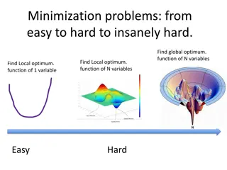
Minimization and Maximization of Functions
Optimization problems involve minimizing or maximizing functions, such as in density functional theory, electronic structure, mechanics, and neural networks. Methods like steepest descent, CG, and BFGS are used in local and global extremum searches. Techniques like bracketing, Taylor expansions, and Golden Section Search help in accurate minimum locating. Parabolic interpolation and Brent's method combine strategies for efficient function optimization.

Download Presentation

Please find below an Image/Link to download the presentation.
The content on the website is provided AS IS for your information and personal use only. It may not be sold, licensed, or shared on other websites without obtaining consent from the author.If you encounter any issues during the download, it is possible that the publisher has removed the file from their server.
You are allowed to download the files provided on this website for personal or commercial use, subject to the condition that they are used lawfully. All files are the property of their respective owners.
The content on the website is provided AS IS for your information and personal use only. It may not be sold, licensed, or shared on other websites without obtaining consent from the author.
E N D
Presentation Transcript
Chapter 10 Minimization or Maximization of Functions
Optimization Problems Solution of an equation can be formulated as an optimization problem, e.g., density functional theory (DFT) in electronic structure, Lagrangian mechanics, determining the weights in neural network, etc Minimization with constraints operations research (linear programming, traveling salesman problem, etc), max entropy with a given energy,
General Consideration Use function values only, or use function values and its derivatives Storage of O(N) or O(N2) With constraints or no constraints Choice of methods Steepest Descent CG BFGS
Bracketing and Search in 1D Bracket a minimum means that for given a < b < c, we have f(b) < f(a), and f(b) < f(c). There is a minimum in the interval (a,c). c a b
How accurate can we locate a minimum? Let b a minimum of function f(x),Taylor expanding around b, we have 1 ( ) ( ) ( )( 2 f b x b + 2 ) f x f b The best we can do is when the second correction term reaches machine epsilon relative accuracy comparing to the function value, so | 2| ( )| ( ) f f b b x b |
Golden Section Search x c a b Choose x such that the ratio of intervals [a,b] to [b,c] is the same as [a,x] to [x,b]. Remove [a,x] if f[x] > f[b], or remove [b,c] if f[x] < f[b]. The asymptotic limit of the ratio is the Golden mean 5 1 2 0.61803
Parabolic Interpolation & Brent s Method 2 ( ) ( ) ( ) ( ) b a f b f c b c b a b c 2 2 ( ) ( ) f b ( ) f c ( ) ( ) ( ) f b ( ) ( ) f a f b f a 1 Brent s method combines parabolic interpolation with Golden section search, with some complicated bookkeeping. See NR, page 404-405 for details. = x b
Minimization as a root-finding problem Let s the derivative dF(x)/dx = f(x), then minimizing (or maximizing) F is the same as finding zero of f, i.e., f(x) = 0. Newton method: approximate curve as a straight line.
Deriving Newton Iteration Let the current value be xn and zero is approximately located at next stop xn+1, using Taylor expansion 0 ( ) ( ) n n f x f x f x + = + + 2 ( )( ) ( ) x x O x + 1 1 n n n Solving for xn+1, we get ( ( ) ) '( ''( ) ) f x f x F x F x += = n n x x x 1 n n n n n
Convergence in Newton Iteration Let x be the exact root, xi is the value in i- th iteration, and i =xi-x is the error, then + = + + 1 2 + ( ) x + 2 3 ( ) ( ) f x ( ) ( ), f x f x f O f x ( ) ( ) x + = + 2 ( ) ( ) f x f O Rate of convergence: ( ), ( ) i f x f x f x f x = i x x + 1 i i f x + + 2 ( ) ( ) ( ) ( ) f x ( )/2 ( ) x f f x = i i i + 1 i i i i i ( ) ( ) f x f x = 2 (Quadratic convergence) i 2
Strategy in Higher Dimensions 1. Starting from a point P and a direction n, find the minimum on the line P + n, i.e., do a 1D minimization of y( )=f(P+ n) 2. Replace P by P + minn, choose another direction n and repeat step 1. The trick and variation of the algorithms are on chosen n.
Local Properties near Minimum Let P be some point of interest which is chosen to be the origin x=0. Taylor expansion gives = + i i x x x 2 1 2 f f i j + + ( ) x ( ) P f f x x x i i j , i j 1 2 c + x T T b x A x Minimizing f is the same as solving the equation = A x b T for transpose of a matrix
Search along Coordinate Directions Search minimum along x direction, followed by search minimum along y direction, and so on. Such a method takes a very large number of steps to converge. The curved loops represent f(x,y) = const.
Steepest Descent Search in the direction with the largest decrease, i.e., n = - f Constant f contour line (surface) is perpendicular to n, because df = dx f = 0. The current search direction n and next search direction are orthogonal, because for minimum we have nT n = 0 n y ( ) = df(P+ n)/d = nT f|P+ n = 0 n
Conjugate Condition Make a linear coordinate transformation, such that contour is circular and (search) vectors are orthogonal n1T A n2 = 0
Conjugate Gradient Method 1. Start with steepest descent direction n0 = g0 = - f(x0), find new minimum x1 2. Build the next search direction n1 from g0 and g1 = - f(x1), such that n0 A n1 = 0 3. Repeat step 2 iteratively to find nj (a Gram-Schmidt orthogonalization process). The result is a set of N vectors (in N dimensions) niT A nj = 0
Conjugate Gradient Algorithm 1. Initialize n0 = g0 = - f(x0), i = 0 2. Find that minimizes f(xi+ ni), let xi+1 =xi+ ni 3. Compute new negative gradient gi+1 = - f(xi+1) 4. Compute i T i g T i g g g = + + 1 1 i (Fletcher-Reeves) i 5. Update new search direction as ni+1 = gi+1 + ini; ++i, go to 2
CG, a Python implementation import numpy as np def conjugate_gradient(A, b, x=None, max_iter=512, reltol=1e-2): if x is None: x=np.zeros_like(b) r=b-A(x) d=r rsnew=np.sum(r.conj()*r).real rs0=rsnew ii=0 while ((ii<max_iter) and (rsnew>(reltol**2*rs0))): ii=ii+1 Ad=A(d) alpha=rsnew/(np.sum(d.conj()*Ad)) x=x+alpha*d if ii%50==0: #every now and then compute exact residual to mitigate # round-off errors r=b-A(x) d=r else: r=r-alpha*Ad rsold=rsnew rsnew=np.sum(r.conj()*r).real d=r+rsnew/rsold*d return x
TensorFlow implementation of CG tf.linalg.experimental.conjugate_gra dient(operator, rhs, preconditioner=None, x=None, tol=1e- 05, max_iterater=20,name= conjugate_grad ient ) Solves a linear system of equations Ax = rhs for Hermitian, positive definite matrix A, the matrix A is presented by operator.
Simulated Annealing To minimize f(x), we make random change to x by the following rule: Set temperature T a large value, decrease as we go Metropolis algorithm: make local change from x to x . If f decreases, accept the change, otherwise, accept only with a small probability r = exp[-(f(x )-f(x))/T]. This is done by comparing r with a random number 0 < < 1.
Traveling Salesman Problem Beijing Tokyo Shanghai Taipei Hong Kong Kuala Lumpur Find shortest path that cycles through each city exactly once. Singapore
Reading Materials Chapter 10 of NR Read: http://www.cs.cmu.edu/~quake- papers/painless-conjugate-gradient.pdf
Problem set 7 (due 28 Oct 2024) 1. Derive the formula of Brent method (minimum x determined by three points): f b 2 2 ( ) ( ) ( ) f b ( ) ( ) f c ( ( ) ) ( ) ( ) ( ) ( ) f a b a b a f b f c b c b c f b f a 1 2 ( = x b ) 2. Suppose that the function is given by the quadratic form f=(1/2)xT A x, where A is a symmetric and positive definite matrix. Find a linear transform to x so that in the new coordinate system, the function becomes f = (1/2)|y|2, y = Ux [i.e., the contour is exactly circular or spherical]. More precisely, give a computational procedure for U. If two vectors in the new system are orthogonal, y1T y2=0, what does it mean in the original system?


")