Model Selection and Assessment in Machine Learning

Model selection and assessment are crucial steps in the machine learning process. Validation is used to select the best model among various options, estimate prediction error, and make informed choices. Analytical approaches and resampling methods help in evaluating model performance and tuning parameters for optimal results.

Download Presentation

Please find below an Image/Link to download the presentation.
The content on the website is provided AS IS for your information and personal use only. It may not be sold, licensed, or shared on other websites without obtaining consent from the author.If you encounter any issues during the download, it is possible that the publisher has removed the file from their server.
You are allowed to download the files provided on this website for personal or commercial use, subject to the condition that they are used lawfully. All files are the property of their respective owners.
The content on the website is provided AS IS for your information and personal use only. It may not be sold, licensed, or shared on other websites without obtaining consent from the author.
E N D
Presentation Transcript
Model Selection and Assessment, Part II Machine Learning, BMTRY 790
Model Assessment Recall we said the best solution Split data into three set Training Set (50% of the sample): Use to build models Validation Set (25% of the sample): Use to validate prediction performance of models developed in training data Test Set (25% of the sample): Used to estimate prediction error on final model selected from first two sets In the event that data are not sufficiently large, there are techniques to estimate model prediction error Mathematical approaches Resampling approaches
Overview: Model Selection The most important use of validation is for model selection For example, this could be: Choosing a regression model from among all possible regression models for p inputs Choice between a linear model and a nonlinear model Choice of a regularization parameter Any other choice that affects statistical learning process. For all prediction modeling, there are choices to be made and we need a consistent way of making these choices. Validation can be used to estimate the out-of-sample error for more than one model.
Analytical Approaches Recall we ve discussed several analytical approaches These methods estimate training error by mathematical adjustment of the training error: Focused on AIC, BIC Typically used in stepwise model fitting approaches Other methods: Minimum description length(MDL) Structural risk minimization (SRM) However, these methods require that we have a way to estimate model complexity, which isn t always the case
Resampling Methods Basic steps Repeatedly draw samples from a training set Fit a model for the outcome of interest on each sample Estimate information about the fitted model Example: Goal: Estimate the variability of a linear regression fit Draw different samples from the training data and fit OLS regression to each Examining the extent to which the resulting fits differ. Can be useful in both model selection and model assessment
Resampling Methods Cross-Validation Useful to tune model parameters Example: Shrinkage parameter l in penalized regression Example: Number of knots in a cubic spline Estimate test set prediction error rates associated with a given method to evaluate its performance Bootstrap Most often used to provide a measure of accuracy of a parameter estimate or of a given statistical or machine learning method.
Overview: Model Selection M1 M2 MM Consider a case where we have M models; validation can be used to select one of these models Training Data 1 y 2 y M y Validation Data Fit models to the training data and evaluate each model on a validation set to obtain the validation errors. Err Err Err T M 2 T 1 T pick the best model Select the model with the lowest validation error ( ) , M Err * * m Tm Full Data Fit selected model to the full data set m y *
K-Fold Cross-Validation General Approach: Randomly split the data into K roughly equal-size subsets. 1 2 K - 1 k K For the kth subset calculate the prediction error of the model fit using the other K 1 subsets. Do this for k = 1, 2, . . . , K and combine the Kestimates of the prediction error.
K-Fold Cross-Validation The mapping of belongs to the th partition indicates observation i : 1,2,..., 1,2,..., N K f-k(x) is the model fitted to the data with the kth subset removed The cross-validation estimate of the prediction error is ( ) CV f N ( ) 1 N ( )( ) i = , L y f x i i = 1 i Typical choices of K include 5 and 10-fold The case where K = N is referred to as leave one out CV
K-Fold Cross-Validation We could also consider statistical models where we need to consider some tuning parameter = shrinkage parameter (penalized regression models) k = number of knots (cubic regression spline In this case, our model function, f(x), is also indexed by the tuning parameter, , as f-k(x, ) Thus the cross-validation estimate of the prediction error is ( ) 1 i N = ( ) 1 N ( )( ) i = , , CV f L y f x i i
Choice of K? Intuition says When K = 5 or 10, then fairly different ( ) CV f Err since training sets from different folds are ( ) When K = N, then since the training sets are very similar for each fold CV f Err T Simulation studies have shown that cross-validation really only effectively estimated Err.
Choice of K? Computation increases Variance decreases bias decreases K fold Leave-one-out K increases
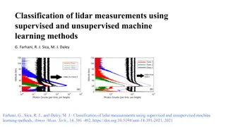
Hypothetical Learning Curve for a Classifier Based on Observed Training Set Sample Size Figure 7.8 from ESL
Choice of K? K = N approximately unbiased estimate of Err. has high variance since the Ntraining sets are similar. Computational burden is high (except for a few exceptions) When K = 5 has low variance. potentially upwardly biased estimate for Err. Only occurs if for each fold there is not enough training data to fit a good model. ( ) ( ) CV f CV f ( ) ( ) CV f CV f K-fold CV with K = 5 orK = 10 shown empirically to yield test error rate estimates that don t suffer from excessively high bias or very high variance.
Generalized Cross-Validation LOOCV can be computationally difficult, particularly in N is large Linear fitting methods with squared error loss can be written as , where S is a smoother matrix For these methods, we can write our LOOCV estimated loss as = y Sy 2 ( ) f x S ( ) y 1 N 1 N N N 2 ( ) x f = i i i y i i 1 = = 1 1 i i ii From this we get the GCV approximation 2 ( ) ( ) S f x ( ) y trace 1 N N = i i GCV f 1 N = 1 i
Conducting CV There are right and wrong ways to do CV. Consider the case where our goal is to develop a multivariable regression model. A wrong strategy: 1. Screen the predictors and find a good subset among the all predictors that are correlated with outcome y. 2. Build a model based on the selected subset of good predictors. 3. Perform cross-validation to estimate the unknown tuning parameters and to estimate Err of the final model.
Conducting CV Better strategy: 1. Divide the data into K randomly selected subsets of data. 2. For each fold k= 1, 2, , K: i. Find the subset of good predictors that show the strongest univariate association with the outcome y minus the kth fold. ii. Using this subset of good predictors, build a multivariate statistical model, again minus the kth fold. iii. Use the model to predict the outcome y in the kth fold. In general, if we are doing multi-step modeling, cross-validation should be applied to the entire sequence of modeling steps.
The Bootstrap Consider training data, Z = {z1, z2, , zN} where zi = {xi, yi}. The bootstrap idea is: For b= 1, 2, , B Randomly select N samples from Z with replacement to yield sample Z*b = * b Z , ,..., 1, 2,..., z z z b N where b b b i 1 2 N Fit a model using Z*b and estimate some statistic of interest S(Z*b) Examine the behavior of the B fits ( ) ( ) ( ) *1 *2 * B Z Z Z , ,..., S S S
Use of Bootstrap to Estimate Distribution of S(Z) From the bootstrap sampling we can estimate any aspect of the distribution of S(Z), for example, its variance: ( ) 1 1 B B ( ) ( ) ( ) 2 ( ) Z = = * * * * b b Z Z Var S S S S S where 1 B = 1 b b While this may be of interest, we really want to get at the prediction error for statistical models
Use of Bootstrap to Estimate Prediction Error We could consider the following to estimate prediction error for our model: 1 boot b i BN = = ( ) B N ( ) x = * b , Err L y f i i 1 1 ( ) x * b f Here is the predicted value at xiusing the model estimated from the bth bootstrap sample, Z i *b Why might this not be a good estimator?
Use of Bootstrap to Estimate Prediction Error Alternatively, we could borrow from the idea of cross-validation Consider only observations not in a bootstrap samples when estimating error Equation for this leave one out bootstrap estimate is 1 i N = ( ) 1 N ( ) x ( ) 1 = * b , Err L y f i i i C i 1 b C C i = set if indices of bootstrap samples bthat don t include observation i |C i | = the number of samples for which this is true Better choice but ( ) ( ) N e = = * 1 b Z 1 1 1 0.632 P i 1 N observation So similar to CV with 2-folds, which as noted earlier may yield high upward bias.
Use of Bootstrap to Estimate Prediction Error The .632 estimators proposed to address bias in the leave one out bootstrap estimate ( ) ( ) 1 .632 = + 0.368 0.632 Err err Err err Here is the training error And is the leave one out bootstrap error Err ( ) 1 Compromise between training and the leave-one-out bootstrap error. Not easy to derive Relates to the probability that an observation is in a bootstrap sample. Does not do well if predictor tends to overfit.
Use of Bootstrap to Estimate Prediction Error The .632 estimator can be improved if we account for the amount of over-fitting First define the no-information error rate as ( ) 1 N N ( ) = , L y f x ' i i 2 N = ' 1 = 1 i i f Estimate of the error rate of if the outcome and predictors were independent. f Note the prediction rule, , is evaluated for all possible combinations of the outcome yi and the predictors xi
Use of Bootstrap to Estimate Prediction Error We can then define the relative over-fitting rate as ( ) 1 Err err = R err R = 0 implies no over-fitting R = 1 implies over-fitting is equal to the no-information error rate minus the training error. 0 < R < 1 implies some evidence of over-fitting with larger values implying more severe over-fitting
Use of Bootstrap to Estimate Prediction Error Depending on amount of over-fitting, the best error estimate is as little as Err(.632), or as much as Err(1) (likely something in between) Err(.632+)is similar to Err(.632)but applies adaptive weights, with Err(1) weighted at least .632 0.632 1 0.368 ( ) ( ) ( ) 1 += .632 + = 1 0 1 Err err Err R where and R Thus Err(.632+)adaptively mixes training error and leave-one-out error using the relative over-fitting rate (R)
Implementing Validation Methods In R Mathematical adjustment of model error (AIC and BIC) stats package Functions that return AIC and BIC for linear models from a variety of other packages Will also fit step-wise regressions and compare based on information criterion MASS package stepAIC function performs step-wise regression based on AIC (very similar to step function from stats package) glmulti package Calculate information criterion (AIC, BIC, QIC) for exhaustive evaluation of set of generalized linear models
Model Selection: Body Fat Example Recall our regression model Call: lm(formula = PBF ~ Age + Wt + Ht + Neck + Chest + Abd + Hip + Thigh + Knee + Ankle + Bicep + Arm + Wrist, data = bodyfat, x = T) Estimate Std. Error t value Pr(>|t|) (Intercept) -18.18849 17.34857 -1.048 0.29551 Age 0.06208 0.03235 1.919 0.05618 . Wt -0.08844 0.05353 -1.652 0.09978 . Ht -0.06959 0.09601 -0.725 0.46925 Neck -0.47060 0.23247 -2.024 0.04405 * Chest -0.02386 0.09915 -0.241 0.81000 Abd 0.95477 0.08645 11.04 < 2e-16 *** Hip -0.20754 0.14591 -1.422 0.15622 Thigh 0.23610 0.14436 1.636 0.10326 Knee 0.01528 0.24198 0.063 0.94970 Ankle 0.17400 0.22147 0.786 0.43285 Bicep 0.18160 0.17113 1.061 0.28966 Arm 0.45202 0.19913 2.270 0.02410 * Wrist -1.62064 0.53495 -3.030 0.00272 ** Residual standard error: 4.305 on 238 degrees of freedom. Multiple R-squared: 0.749, Adjusted R-squared: 0.7353 . F-statistic: 54.65 on 13 and 238 DF, p-value: < 2.2e-16
Model Selection: Body Fat Example ### Regression Data Example bodyfat<-read.csv("H:/public_html/BMTRY790_Spring2023/Datasets/Body_fat.csv") bodyfat<-bodyfat[,2:15] ### Extracting AIC and BIC from single models mod1<-lm(PBF ~ ., data=bodyfat) AIC(mod1) [1] 1466.502 BIC(mod1) [1] 1519.444
Model Selection: Body Fat Example ### Forward selection using AIC with step/stepAIC function mod1<-lm(PBF ~ ., data=bodyfat) nmod1<-lm(PBF ~ 1, data=bodyfat) fmod1a<-step(nmod1, scope=list(lower=nmod1, upper=mod1), direction="forward") Start: AIC=1071.75 PBF ~ 1 Df Sum of Sq RSS AIC + Abd 1 11631.5 5947.5 800.65 + Chest 1 8678.3 8900.7 902.24 Step: AIC=741.85 PBF ~ Abd + Wt + Wrist + Arm + Neck + Age + Thigh + Hip Df Sum of Sq RSS AIC <none> 4455.3 741.85 + Bicep 1 20.7116 4434.6 742.68 + Ht 1 11.7494 4443.6 743.19 + Ankle 1 11.6199 4443.7 743.19 + Knee 1 0.0365 4455.3 743.85 + Chest 1 0.0001 4455.3 743.85
Model Selection: Body Fat Example ### Forward selection using AIC with step/stepAIC function names(fmod1a) [1] "coefficients" "residuals" "effects" "rank" "fitted.values" "assign" "qr" "df.residual" "xlevels" "call" [2] "terms" "model" "anova" fmod1a$coef (Intercept) Abd Wt Wrist Arm Neck Age Thigh Hip -22.65637291 0.94481514 -0.08985290 -1.53665172 0.51572117 -0.46655783 0.06577964 0.30239157 -0.19543492 fmod1a$anova Step Df Deviance Resid. Df Resid. Dev AIC 1 NA NA 251 17578.990 1071.7477 2 + Abd -1 11631.52681 250 5947.463 800.6453 3 + Wt -1 1004.21778 249 4943.245 756.0398 4 + Wrist -1 157.19103 248 4786.054 749.8962 5 + Arm -1 127.81846 247 4658.236 745.0747 6 + Neck -1 51.06638 246 4607.169 744.2968 7 + Age -1 47.93419 245 4559.235 743.6612 8 + Thigh -1 67.38659 244 4491.849 741.9088 9 + Hip -1 36.52435 243 4455.324 741.8514
Model Selection: Body Fat Example ### Backward selection using AIC with step/stepAIC function fmod1b<-step(mod1, direction="backward") fmod1b$coef (Intercept) Age Wt Neck Abd Hip Thigh Arm -22.65637291 0.06577964 -0.08985290 -0.46655783 0.94481514 -0.19543492 0.30239157 0.51572117 Wrist -1.53665172 fmod1b$anova Step Df Deviance Resid. Df Resid. Dev AIC 1 NA NA 238 4411.448 749.3574 2 - Knee 1 0.07392147 239 4411.522 747.3616 3 - Chest 1 1.13294221 240 4412.655 745.4263 4 - Ht 1 8.67544475 241 4421.330 743.9212 5 - Ankle 1 13.28231735 242 4434.613 742.6772 6 - Bicep 1 20.71159705 243 4455.324 741.8514
Model Selection: Body Fat Example ### Forward-Backward selection using AIC with step/stepAIC function fmod1c<-step(mod1, direction="both") fmod1c$coef (Intercept) Age Wt Neck Abd Hip Thigh Arm -22.65637291 0.06577964 -0.08985290 -0.46655783 0.94481514 -0.19543492 0.30239157 0.51572117 Wrist -1.53665172 fmod1c$anova Step Df Deviance Resid. Df Resid. Dev AIC 1 NA NA 238 4411.448 749.3574 2 - Knee 1 0.07392147 239 4411.522 747.3616 3 - Chest 1 1.13294221 240 4412.655 745.4263 4 - Ht 1 8.67544475 241 4421.330 743.9212 5 - Ankle 1 13.28231735 242 4434.613 742.6772 6 - Bicep 1 20.71159705 243 4455.324 741.8514
Model Selection: Body Fat Example ### Forward-Backward selection using BIC with step/stepAIC function n<-nrow(bodyfat) fmod1d<-step(mod1, direction="both", k=log(n)) fmod1d$coef (Intercept) Wt Abd Arm Wrist -34.8540743 -0.1356315 0.9957513 0.4729284 -1.5055620 fmod1d$anova Step Df Deviance Resid. Df Resid. Dev AIC 1 NA NA 238 4411.448 798.7694 2 - Knee 1 0.07392147 239 4411.522 793.2442 3 - Chest 1 1.13294221 240 4412.655 787.7794 4 - Ht 1 8.67544475 241 4421.330 782.7450 5 - Ankle 1 13.28231735 242 4434.613 777.9714 6 - Bicep 1 20.71159705 243 4455.324 773.6162 7 - Hip 1 36.52434618 244 4491.849 770.1442 8 - Neck 1 61.67131402 245 4553.520 768.0511 9 - Thigh 1 66.35368037 246 4619.874 766.1673 10 - Age 1 38.36216099 247 4658.236 762.7218
Model Selection: Breast Carcinoma Consider the logistic regression model Call: glm(formula = Iclass ~ ., family = "binomial", data = btis[, -c(1:2, 9)]) Deviance Residuals: Min 1Q Median 3Q Max -1.78712 -0.13268 -0.01431 0.00000 2.42565 Estimate Std. Error z value Pr(>|z|) (Intercept) 22.0599 16.1578 1.365 0.1722 I0 -0.1868 0.1136 -1.644 0.1001 PA500 -133.4658 90.9269 -1.468 0.1421 HFS -49.3899 27.2195 -1.815 0.0696 . normArea -0.1020 0.2715 -0.376 0.7071 MaxIP 0.9928 0.6454 1.538 0.1240 DR 0.2647 0.1590 1.665 0.0960 . (Dispersion parameter for binomial family taken to be 1) Null deviance: 94.472 on 83 degrees of freedom Residual deviance: 17.382 on 77 degrees of freedom AIC: 31.382 Number of Fisher Scoring iterations: 11 >
Model Selection: Breast Carcinoma ### Classification Example btis<-read.csv("H:\\public_html\\BMTRY790_Spring2023\\Datasets\\BreastTissue.csv") btis<-btis[-which(btis$Class=="adipose"),] btis$Iclass<-ifelse(btis$Class=="carcinoma", 1, 0) mod2<-glm(Iclass ~ ., data=btis[,-c(1:2,8,9)], family="binomial") AIC(mod2) [1] 31.38202 BIC(mod2) [1] 48.39773
Model Selection: Breast Carcinoma ### Forward-Backward selection using AIC with step/stepAIC function mod2<-glm(Iclass ~ ., data=btis[,-c(1:2,9)], family="binomial") fmod2c<-step(mod2, direction="both") fmod2c$coef (Intercept) I0 PA500 HFS MaxIP DR 17.6046346 -0.1546919 -110.3712274 -43.7315077 0.7977925 0.2215606 fmod2c$anova Step Df Deviance Resid. Df Resid. Dev AIC 1 NA NA 77 17.38202 31.38202 2 - normArea 1 0.14728 78 17.52930 29.52930
Implementing Validation Methods In R Resampling methods DAAG package (Data Analysis and Graphics Data and Functions) Provides cross-validation function for linear and logistic regression models. cvTools package Provides functions to estimate cross-validation error for regression models Bootstrap package Provides functions for cross-validation, bootstrapping, and jackknifing e1071 package Provides function to tune model fit parameters for neural net, SVM, CART, random forest, and kNN models caret package Provides unified framework for running model validation via resampling for a variety of model types available in R Able to select different types of cross-validation or bootstrap resampling validation methods Provides user ability to set a specific model evaluation function
Model Selection: Body Fat Example ### Regression Data Example library(caret) tmod1.cv1<-train(PBF ~ ., data=bodyfat, trControl=trainControl("cv", number=10), method="glmStepAIC") names(tmod1.cv1) [1] "method" "modelInfo" "modelType" "results" "pred" "bestTune" "call" [8] "dots" "metric" "control" "finalModel" "preProcess" "trainingData" "resample" [15] "resampledCM" "perfNames" "maximize" "yLimits" "times" "levels" "terms" [22] "coefnames" "xlevels"
Model Selection: Body Fat Example ### Regression Data Example, 10-fold CV tmod1.cv1$results parameter RMSE Rsquared RMSESD RsquaredSD 1 none 4.399959 0.7346191 0.6194202 0.08389727 tmod1.cv1$resample RMSE Rsquared parameter Resample 1 4.545380 0.6634375 none Fold01 2 4.473056 0.7219830 none Fold02 9 4.953042 0.7037010 none Fold09 10 3.091050 0.8593599 none Fold10 tmod1.cv1$finalModel Call: NULL Coefficients: (Intercept) Age Wt Neck Abd Hip Thigh Arm Wrist -22.65637 0.06578 -0.08985 -0.46656 0.94482 -0.19543 0.30239 0.51572 -1.53665 Degrees of Freedom: 251 Total (i.e. Null); 243 Residual Null Deviance: 17580 Residual Deviance: 4455 AIC: 1459
Model Selection: Body Fat Example ### Regression Data Example- Leave one out CV tmod1.cv2<-train(PBF ~ ., data=bodyfat, trControl=trainControl("loocv", returnResamp="all"), method="glmStepAIC") tmod1.cv2$results parameter RMSE Rsquared RMSESD RsquaredSD 1 none 3.708457 NaN 2.564497 NA tmod1.cv2$resample RMSE Rsquared parameter Resample 1 3.639318251 NA none Fold001 2 3.295423590 NA none Fold002 251 1.573132933 NA none Fold251 252 4.837298106 NA none Fold252 tmod1.cv2$finalModel Coefficients: (Intercept) Age Wt Neck Abd Hip Thigh Arm Wrist -22.65637 0.06578 -0.08985 -0.46656 0.94482 -0.19543 0.30239 0.51572 -1.53665 Degrees of Freedom: 251 Total (i.e. Null); 243 Residual Null Deviance: 17580 Residual Deviance: 4455 AIC: 1459
Model Selection: Body Fat Example ### Regression Data Example-Bootstrap resampling tmod1.bs1<-train(PBF ~ ., data=bodyfat, trControl=trainControl("boot", number=100, returnResamp="all"), method="glmStepAIC") tmod1.bs1$results parameter RMSE Rsquared RMSESD RsquaredSD 1 none 4.65436 0.7013852 0.3221535 0.04098558 tmod1.bs1$resample RMSE Rsquared parameter Resample 1 4.542549 0.6317638 none Resample001 2 4.606437 0.6752286 none Resample002 99 4.333208 0.7067568 none Resample099 100 4.529748 0.6724845 none Resample100 tmod1.bs1$finalModel Coefficients: (Intercept) Age Wt Neck Abd Hip Thigh Arm Wrist -22.65637 0.06578 -0.08985 -0.46656 0.94482 -0.19543 0.30239 0.51572 -1.53665 Degrees of Freedom: 251 Total (i.e. Null); 243 Residual Null Deviance: 17580 Residual Deviance: 4455 AIC: 1459
Model Selection: Body Fat Example ### Regression Data Example- .632 Bootstrap and adaptive Bootstrap tmod1.bs2<-train(PBF ~ ., data=bodyfat, trControl=trainControl("boot632", number=1000), method="glmStepAIC") tmod1.bs2$results tmod1.bs2$resample tmod1.bs2$finalModel tmod1.bs3<-train(PBF ~ ., data=bodyfat, trControl=trainControl("adaptive_boot", number=1000), method="glmStepAIC") tmod1.bs3$results tmod1.bs3$resample tmod1.bs3$finalModel
Model Selection: Body Fat Example ### What about direction of selection? ### Backward (default) back.cv<-train(x=bodyfat[,2:14], y=bodyfat[,1], trControl=trainControl("cv", number=10), method="glmStepAIC") ### Forward for.cv<-train(x=bodyfat[,2:14], y=bodyfat[,1], trControl=trainControl("cv", number=10), method="glmStepAIC", direction="forward") ### Forward-Backward both.cv<-train(x=bodyfat[,2:14], y=bodyfat[,1], trControl=trainControl("cv", number=10), method="glmStepAIC", direction="both")
Classification Model Selection: Breast Carcinoma ### Also using step AIC but for GLM model tmod2.cv1<-train(x=btis[,3:7], y=as.factor(btis[,10]), trControl=trainControl("cv", number=10), metric="Accuracy", method="glmStepAIC", family="binomial") tmod2.cv1$results parameter Accuracy Kappa AccuracySD KappaSD 1 none 0.9163889 0.7878401 0.08287373 0.1958306 tmod2.cv1$resample Accuracy Kappa Resample 1 0.8750000 0.7142857 Fold01 2 1.0000000 1.0000000 Fold02 3 1.0000000 1.0000000 Fold03 4 0.8750000 0.6000000 Fold04 5 0.9000000 0.7368421 Fold05 6 1.0000000 1.0000000 Fold06 7 0.8750000 0.6000000 Fold07 8 0.7500000 0.5000000 Fold08 9 0.8888889 0.7272727 Fold09 10 1.0000000 1.0000000 Fold10
Classification Model Selection: Breast Carcinoma ### Also using step AIC but for GLM model tmod2.cv1$finalModel Call: NULL Coefficients: (Intercept) PA500 normArea -9.5550 38.1756 0.1181 Degrees of Freedom: 83 Total (i.e. Null); 81 Residual Null Deviance: 94.47 Residual Deviance: 30.24 AIC: 36.24 confusionMatrix(tmod2.cv1) Cross-Validated (10 fold) Confusion Matrix (entries are percentual average cell counts across resamples) Reference Prediction 0 1 0 70.2 3.6 1 4.8 21.4 Accuracy (average) : 0.9167
Thermoregulation During Surgery Occurrence of hypothermia during surgery is associated with increased complication rate Hypothermia defined as temperature < 36.0oC The goal of the study was to identify patient/hospital factors associated with hypothermia to identify potential interventions Information collected in the study included Patient characteristics (gender, age, BMI) Procedural characteristics (surgery, anesthesia type, EBL, Total IV Fluids) Hospital characteristics (matress temperature, OR temperature, OR humidity) Time in surgery
Using K-Fold CV to Tune Cubic Spline ### 10-fold cross-validation set.seed(12345) cv.ids<-sample(1:370, 370, replace=F) temp2<-temp[cv.ids]; time2<-time[cv.ids] vecmat<-matrix(1:370, nrow=37, ncol=10, byrow=F) cv.err<-matrix(nrow=10, ncol=7) for(i in 1:10){ ids<-vecmat[,i] trtemp<-temp2[-ids]; tstemp<-temp2[ids] trtime<-time2[-ids]; tstime<-time2[ids] for (j in 1:7) { fit<-lm(trtemp ~ ns(trtime, df=(j+3))) cv.err[i,j]<-mean((temp2[ids]-predict(fit, newdata=data.frame(trtime=tstime)))^2) } } round(colMeans(cv.err), 4) [1] 0.3106 0.3120 0.3136 0.3124 0.3147 0.3126 0.3176
Using LOOCV to Tune Cubic Spline ### Leave one out cross-validation cv.err2<-matrix(nrow=length(time), ncol=7) for(i in 1:length(time)) { trtemp<-temp[-i]; tstemp<-temp[i] trtime<-time[-i]; tstime<-time[i] for (j in 1:7) { fit<-lm(trtemp ~ ns(trtime, df=(j+3))) cv.err2[i,j]<-(tstemp-predict(fit, newdata=data.frame(trtime=tstime)))^2 } } round(colMeans(cv.err2), 4) [1] 0.3095 0.3100 0.3108 0.3115 0.3123 0.3101 0.3116
Using Bootstrap Sampling to Tune Cubic Spline ### Bootstrap validation nboot<-1000 berrs<-vector("list", length=7) berrs[[1]]<-berrs[[2]]<-berrs[[3]]<-berrs[[4]]<-berrs[[5]]<-berrs[[6]]<-berrs[[7]]<-sids<- matrix(0, nrow=length(time), ncol=nboot) set.seed(12345) for(i in 1:nboot) { ibids<-sample(1:length(time), length(time), replace=T) nibids<-c(1:length(time))[-unique(ibids)] sids[nibids,i]<-1 trtemp<-temp[ibids]; tstemp<-temp[nibids] trtime<-time[ibids]; tstime<-time[nibids] for (j in 1:7) { fit<-lm(trtemp ~ ns(trtime, df=(j+3))) berrs[[j]][nibids,i]<-(tstemp-predict(fit, newdata=data.frame(trtime=tstime)))^2 } } bootsum<-function(x) {mbserr<-mean(colSums(x)/colSums(sids))} round(unlist(lapply(berrs, bootsum)), 4) [1] 0.3143 0.3154 0.3169 0.3185 0.3197 0.3192 0.3213


")