Multiple Regression Analysis for Data Interpretation
Explore the concept of multiple regression analysis, where various explanatory variables collectively explain a response variable. Dr. Mohammed Alahmed delves into distribution patterns, model examples, and parameter estimation methods. Gain insights into complex regression modeling for data analysis.

Download Presentation

Please find below an Image/Link to download the presentation.
The content on the website is provided AS IS for your information and personal use only. It may not be sold, licensed, or shared on other websites without obtaining consent from the author. If you encounter any issues during the download, it is possible that the publisher has removed the file from their server.
You are allowed to download the files provided on this website for personal or commercial use, subject to the condition that they are used lawfully. All files are the property of their respective owners.
The content on the website is provided AS IS for your information and personal use only. It may not be sold, licensed, or shared on other websites without obtaining consent from the author.
E N D
Presentation Transcript
Multiple Regression Analysis Dr. mohammed Alahmed Dr. Mohammed Alahmed http://fac.ksu.edu.sa/alahmed alahmed@ksu.edu.sa (011) 4674108 1
Introduction In simple linear regression we studied the relationship between one explanatory variable and one response variable. Now, we look at situations where several explanatory variables works together to explain the response. Dr. mohammed Alahmed 2
Introduction Following our principles of data analysis, we look first at each variable separately, then at relationships among the variables. Dr. mohammed Alahmed We look at the distribution of each variable to be used in multiple regression to determine if there are any unusual patterns that may be important in building our regression analysis. 3
Multiple Regression Example: In a study of direct operating cost, Y, for 67 branch offices of consumer finance charge, four independent variables were considered: X1 : average size of loan outstanding during the year, X2 : average number of loans outstanding, X3 : total number of new loan applications processed, and X4 : office salary scale index. The model for this example is + + = 2 1 1 0 x x Y Dr. mohammed Alahmed + + + X x 2 3 3 4 4 4
Formal Statement of the Model General regression model = + + + + + Y x x kx 0 1 1 2 2 k Dr. mohammed Alahmed Where: 0, 1, , k are parameters X1, X2, ,Xk are known constants , the error terms are independent N(o, 2) 5
Estimating the parameters of the model The values of the regression parameters i are not known. We estimate them from data. As in the simple linear regression case, we use the least-squares method to fit a linear function to the data. b x b b y + + = 1 1 0 Dr. mohammed Alahmed + + x b kx 2 2 k The least-squares method chooses the b s that make the sum of squares of the residuals as small as possible. 6
Estimating the parameters of the model The least-squares estimates are the values that minimize the quantity = i n 2 y ( ) y i i Dr. mohammed Alahmed 1 Since the formulas for the least-squares estimates are complicated and hand calculation is out of question, we are content to understand the least- squares principle and let software do the computations. 7
Estimating the parameters of the model The estimate of i is bi and it indicates the change in the mean response per unit increase in Xi when the rest of the independent variables in the model are held constant. The parameters i are frequently called partial regression coefficients because they reflect the partial effect of one independent variable when the rest of independent variables are included in the model and are held constant Dr. mohammed Alahmed 8
Estimating the parameters of the model The observed variability of the responses about this fitted model is measured by the variance: 1 n = i = 2 2 y ( ) S y Dr. mohammed Alahmed i i 1 n k 1 and the regression standard error: s = 2s 9
Estimating the parameters of the model In the model 2 and measure the variability of the responses about the population regression equation. It is natural to estimate 2 by s2 and by s. Dr. mohammed Alahmed 10
Analysis of Variance Table The basic idea of the regression ANOVA table are the same in simple and multiple regression. The sum of squares decomposition and the associated degrees of freedom are: ( ) ( Dr. mohammed Alahmed = + 2 2 2 y ) ( ) y y y y y i i i i = + SST SSR SSE df: = + ) 1 1 ( n k n k 11
Analysis of Variance Table Sum of Squares SS Mean Square MS Source df F-test Dr. mohammed Alahmed MSR= SSR/k MSE= SSE/n-k-1 Regression SSR MSR/MSE k Error SSE n-k-1 Total SST n-1 12
F-test for the overall fit of the model To test the statistical significance of the regression relation between the response variable y and the set of variables x1, , xk, i.e. to choose between the alternatives: = = = = Dr. mohammed Alahmed : 0 H 0 1 2 k = : not all ( , 1 equal ) zero H i k a i We use the test statistic: MSR F = MSE 13
F-test for the overall fit of the model The decision rule at significance level is: Reject H0 if F F ) 1 ( ; , k n k Where the critical value F( , k, n-k-1) can be found from an F-table. The existence of a regression relation by itself does not assure that useful prediction can be made by using it. Note that when k=1, this test reduces to the F-test for testing in simple linear regression whether or not 1= 0 Dr. mohammed Alahmed 14
Interval estimation of i For our regression model, we have: b has a t - distributi on with n - degrees 1 - k of freedom i s i (i b ) Therefore, an interval estimate for i with 1- confidence coefficient is: Where = ( x Dr. mohammed Alahmed ( ) ( ) b t s b ; 1 n k i i 2 MSE ( ) s b i 2) x 15
Significance tests for i = To test: : 0 H 0 i : 0 H a i We may use the test statistic: Dr. mohammed Alahmed b t = i (i b ) s Reject H0 if ) 1 ( ; t t n k or 2 16 ) 1 ( ; t t n k 2
Multiple regression model Building Often we have many explanatory variables, and our goal is to use these to explain the variation in the response variable. A model using just a few of the variables often predicts about as well as the model using all the explanatory variables. Dr. mohammed Alahmed 17
Multiple regression model Building We may find that the reciprocal of a variable is a better choice than the variable itself, or that including the square of an explanatory variable improves prediction. We may find that the effect of one explanatory variable may depends upon the value of another explanatory variable. We account for this situation by including interaction terms. Dr. mohammed Alahmed 18
Multiple regression model Building The simplest way to construct an interaction term is to multiply the two explanatory variables together. How can we find a good model? Dr. mohammed Alahmed 19
Selecting the best Regression equation. After a lengthy list of potentially useful independent variables has been compiled, some of the independent variables can be screened out. An independent variable May not be fundamental to the problem May be subject to large measurement error May effectively duplicate another independent variable in the list. Dr. mohammed Alahmed 20
Selecting the best Regression Equation. Once the investigator has tentatively decided upon the functional forms of the regression relations (linear, quadratic, etc.), the next step is to obtain a subset of the explanatory variables (x) that best explain the variability in the response variable y. Dr. mohammed Alahmed 21
Selecting the best Regression Equation. An automatic search procedure that develops sequentially the subset of explanatory variables to be included in the regression model is called stepwise procedure. It was developed to economize on computational efforts. It will end with the identification of a single regression model as best . Dr. mohammed Alahmed 22
Example: Sales Forecasting Sales Forecasting Multiple regression is a popular technique for predicting product sales with the help of other variables that are likely to have a bearing on sales. Example The growth of cable television has created vast new potential in the home entertainment business. The following table gives the values of several variables measured in a random sample of 20 local television stations which offer their programming to cable subscribers. A TV industry analyst wants to build a statistical model for predicting the number of subscribers that a cable station can expect. Dr. mohammed Alahmed 23
Example: Sales Forecasting Y = Number of cable subscribers (SUSCRIB) X1 = Advertising rate which the station charges local advertisers for one minute of prim time space (ADRATE) X2= Number of families living in the station s area of dominant influence (ADI), a geographical division of radio and TV audiences (APIPOP) X3 = Number of competing stations in the ADI (COMPETE) X4= Kilowatt power of the station s non-cable signal (SIGNAL) Dr. mohammed Alahmed 24
Example: Sales Forecasting The sample data are fitted by a multiple regression model using Excel program. The marginal t-test provides a way of choosing the variables for inclusion in the equation. The fitted Model is Dr. mohammed Alahmed = + + + + SUBSCRIBE ADRATE APIPOP COMPETE SIGNAL 0 1 2 3 4 25
Example: Sales Forecasting Excel Summary output SUMMARY OUTPUT Regression Statistics Multiple R R Square Adjusted R Square Standard Error Observations 0.884267744 0.781929444 0.723777295 142.9354188 Dr. mohammed Alahmed 20 ANOVA df SS MS F Significance F 7.52E-05 Regression Residual Total 4 1098857.84 306458.0092 1405315.85 274714.4601 13.44626923 20430.53395 15 19 Coefficients 51.42007002 -0.267196347 -0.020105139 0.440333955 16.230071 Standard Error 98.97458277 0.081055107 -3.296477624 0.004894126 0.045184758 -0.444954014 0.662706578 0.135200486 3.256896248 0.005307766 26.47854322 0.61295181 0.549089662 t Stat 0.51952803 0.610973806 P-value Lower 95%Upper 95% -159.539 -0.43996 -0.11641 0.152161 -40.2076 Intercept AD_Rate Signal APIPOP Compete 262.3795 -0.09443 0.076204 0.728507 72.66778 26
Example: Sales Forecasting Do we need all the four variables in the model? Based on the partial t-test, the variables signal and compete are the least significant variables in our model. Let s drop the least significant variables one at a time. Dr. mohammed Alahmed 27
Example: Sales Forecasting Excel Summary Output SUMMARY OUTPUT Regression Statistics Multiple R R Square Adjusted R Square Standard Error Observations 0.882638739 0.779051144 0.737623233 139.3069743 Dr. mohammed Alahmed 20 ANOVA df SS MS F Significance F 1.69966E-05 Regression Residual Total 3 1094812.92 310502.9296 1405315.85 364937.64 18.80498277 19406.4331 16 19 Coefficients 51.31610447 -0.259538026 0.433505145 13.92154404 Standard Error 96.4618242 0.531983558 0.602046756 0.077195983 -3.36206646 0.003965102 0.130916687 3.311305499 0.004412929 25.30614013 0.550125146 0.589831583 t Stat P-value Lower 95% -153.1737817 -0.423186162 0.15597423 -39.72506442 67.56815 Upper 95% 255.806 -0.09589 0.711036 Intercept AD_Rate APIPOP Compete 28
Example: Sales Forecasting The variable Compete is the next variable to get rid of. Dr. mohammed Alahmed 29
Example: Sales Forecasting Excel Summary Output SUMMARY OUTPUT Regression Statistics Multiple R R Square Adjusted R Square Standard Error Observations 0.8802681 0.774871928 0.748386273 136.4197776 Dr. mohammed Alahmed 20 ANOVA df SS MS F Significance F 3.13078E-06 Regression Residual Total 2 1088939.802 316376.0474 1405315.85 544469.901 18610.35573 29.2562866 17 19 Coefficients 96.28121395 -0.254280696 0.495481252 Standard Error 50.16415506 0.075014548 -3.389751739 0.065306012 t Stat P-value 0.07188916 0.003484198 7.45293E-07 Lower 95% -9.556049653 -0.41254778 -0.096013612 0.357697418 Upper 95% 202.1184776 Intercept AD_Rate APIPOP 1.919322948 7.587069489 0.633265086 30
Example: Sales Forecasting All the variables in the model are statistically significant, therefore our final model is: Final Model Dr. mohammed Alahmed = + SUBSCRIBE 96 28 . . 0 25 ADRATE . 0 495 APIPOP 31
Interpreting the Final Model What is the interpretation of the estimated parameters. Is the association positive or negative? Does this make sense intuitively, based on what the data represents? What other variables could be confounders? Are there other analysis that you might consider doing? New questions raised? Dr. mohammed Alahmed 32
Multicollinearity In multiple regression analysis, one is often concerned with the nature and significance of the relations between the explanatory variables and the response variable. Questions that are frequently asked are: 1. What is the relative importance of the effects of the different independent variables? 2. What is the magnitude of the effect of a given independent variable on the dependent variable? Dr. mohammed Alahmed 33
Multicollinearity 3. Can any independent variable be dropped from the model because it has little or no effect on the dependent variable? 4. Should any independent variables not yet included in the model be considered for possible inclusion? Simple answers can be given to these questions if: The independent variables in the model are uncorrelated among themselves. They are uncorrelated with any other independent variables that are related to the dependent variable but omitted from the model. Dr. mohammed Alahmed 34
Multicollinearity When the independent variables are correlated among themselves, multicollinearity or colinearity among them is said to exist. In many non-experimental situations in business, economics, and the social and biological sciences, the independent variables tend to be correlated among themselves. For example, in a regression of family food expenditures on the variables: family income, family savings, and the age of head of household, the explanatory variables will be correlated among themselves. Dr. mohammed Alahmed 35
Multicollinearity Further, the explanatory variables will also be correlated with other socioeconomic variables not included in the model that do affect family food expenditures, such as family size. Dr. mohammed Alahmed 36
Multicollinearity Some key problems that typically arise when the explanatory variables being considered for the regression model are highly correlated among themselves are: 1. Adding or deleting an explanatory variable changes the regression coefficients. 2. The estimated standard deviations of the regression coefficients become large when the explanatory variables in the regression model are highly correlated with each other. 3. The estimated regression coefficients individually may not be statistically significant even though a definite statistical relation exists between the response variable and the set of explanatory variables. Dr. mohammed Alahmed 37
Multicollinearity Diagnostics A formal method of detecting the presence of multicollinearity that is widely used is by the means of Variance Inflation Factor. It measures how much the variances of the estimated regression coefficients are inflated as compared to when the independent variables are not linearly related. Dr. mohammed Alahmed 1 = , 2 , 1 = , VIF j k j 2 1 R j 2 j R is the coefficient of determination from the regression of the jth independent variable on the remaining k-1 independent variables. 38
Multicollinearity Diagnostics VIF near 1 suggests that multicollinearity is not a problem for the independent variables. - Its estimated coefficient and associated t-value will not change much as the other independent variables are added or deleted from the regression equation. VIF much greater than 1 indicates the presence of multicollinearity. A maximum VIF value in excess of 10 is often taken as an indication that the multicollinearity may be unduly influencing the least square estimates. - the estimated coefficient attached to the variable is unstable and its associated t statistic may change considerably as the other independent variables are added or deleted. Dr. mohammed Alahmed 39
Multicollinearity Diagnostics The simple correlation coefficient between all pairs of explanatory variables (i.e., X1, X2, , Xk ) is helpful in selecting appropriate explanatory variables for a regression model and is also critical for examining multicollinearity. Dr. mohammed Alahmed While it is true that a correlation very close to +1 or 1 does suggest multicollinearity, it is not true (unless there are only two explanatory variables) to infer multicollinearity does not exist when there are no high correlations between any pair of explanatory variables. 40
Example: Sales Forecasting Pearson Correlation Coefficients, N = 20 Prob > |r| under H0: Rho=0 SUBSCRIB ADRATE KILOWATT APIPOP COMPETE SUBSCRIB 1.00000 -0.02848 0.44762 0.90447 0.79832 SUBSCRIB 0.9051 0.0478 <.0001 <.0001 ADRATE -0.02848 1.00000 -0.01021 0.32512 0.34147 ADRATE 0.9051 0.9659 0.1619 0.1406 Dr. mohammed Alahmed SIGNAL SIGNAL 0.44762 -0.01021 1.00000 0.45303 0.46895 0.0478 0.9659 0.0449 0.0370 APIPOP 0.90447 0.32512 0.45303 1.00000 0.87592 APIPOP <.0001 0.1619 0.0449 <.0001 COMPETE 0.79832 0.34147 0.46895 0.87592 1.00000 COMPETE <.0001 0.1406 0.0370 <.0001 41
Example: Sales Forecasting = + + SUBSCRIBE 51 42 . . 0 27 ADRATE - .02 SIGNAL . 0 44 APIPOP 16.23 COMPETE = + + SUBSCRIBE 51 32 . . 0 26 ADRATE . 0 43 APIPOP 13.92 COMPETE Dr. mohammed Alahmed = + SUBSCRIBE 96 28 . . 0 25 ADRATE . 0 495 APIPOP 42
Example: Sales Forecasting VIF calculation: Fit the model APIPOP = + + + SIGNAL ADRATE COMPETE 0 1 2 3 SUMMARY OUTPUT Dr. mohammed Alahmed Regression Statistics Multiple R R Square Adjusted R Square Standard Error Observations 0.878054 0.770978 0.728036 264.3027 20 ANOVA df SS MS 1254200 69855.92 F Significance F 2.25472E-05 Regression Residual Total 3 3762601 1117695 4880295 17.9541 16 19 Coefficients -472.685 159.8413 0.048173 0.037937 Standard Error t Stat 139.7492 28.29157 0.149395 0.083011 P-value 0.003799 3.62E-05 0.751283 0.653806 Lower 95% -768.9402258 99.86587622 -0.268529713 -0.138038952 Upper 95% -176.43 219.8168 0.364876 0.213913 43 Intercept Compete ADRATE Signal -3.38238 5.649786 0.322455 0.457012
Example: Sales Forecasting Fit the model Compete = + + + ADRATE APIPOP SIGNAL 0 1 2 3 SUMMARY OUTPUT Regression Statistics Multiple R R Square Adjusted R Square Standard Error Observations Dr. mohammed Alahmed 0.882936 0.779575 0.738246 1.34954 20 ANOVA df SS MS F Significance F 1.66815E-05 Regression Residual Total 3 103.0599 29.14013 132.2 34.35329 1.821258 18.86239 16 19 Coefficients 3.10416 0.000491 0.000334 0.004167 Standard Error t Stat 0.520589 0.000755 0.000418 0.000738 P-value 1.99E-05 0.525337 0.435846 3.62E-05 Lower 95% 2.000559786 -0.001110874 -0.000552489 0.002603667 Upper 95% 4.20776 0.002092 0.001221 0.005731 Intercept ADRATE Signal APIPOP 5.96278 0.649331 0.799258 5.649786 44
Example: Sales Forecasting Fit the model = + + + Signal ADRATE APIPOP COMPETE 0 1 2 3 SUMMARY OUTPUT Regression Statistics Multiple R R Square Adjusted R Square Standard Error Observations Dr. mohammed Alahmed 0.512244 0.262394 0.124092 790.8387 20 ANOVA df SS MS 1186596 625425.8 F Significance F 0.170774675 Regression Residual Total 3 3559789 1.897261 16 10006813 19 13566602 Coefficients 5.171093 0.339655 114.8227 -0.38091 Standard Error t Stat 547.6089 0.743207 143.6617 0.438238 P-value 0.992582 0.653806 0.435846 0.397593 Lower 95% -1155.707711 -1.235874129 -189.7263711 -1.309935875 Upper 95% 1166.05 1.915184 419.3718 0.548109 Intercept APIPOP Compete ADRATE 0.009443 0.457012 0.799258 -0.86919 45
Example: Sales Forecasting Fit the model = + + + ADRATE Signal APIPOP COMPETE 0 1 2 3 SUMMARY OUTPUT Regression Statistics Multiple R R Square Adjusted R Square Standard Error Observations Dr. mohammed Alahmed 0.399084 0.159268 0.001631 440.8588 20 ANOVA df SS MS F Significance F 0.413876018 Regression Residual Total 3 589101.7 3109703 3698805 196367.2 194356.5 1.010346 16 19 Coefficients 253.7304 -0.11837 0.134029 52.3446 Standard Error t Stat 298.6063 0.136186 0.415653 80.61309 P-value 0.408018 0.397593 0.751283 0.525337 Lower 95% -379.2865355 -0.407073832 -0.747116077 -118.5474784 Upper 95% 886.7474 0.170329 1.015175 223.2367 Intercept Signal APIPOP Compete 0.849716 -0.86919 0.322455 0.649331 46
Example: Sales Forecasting VIF calculation Results: Variable ADRATE COMPETE SIGNAL APIPOP R- Squared 0.159268 0.779575 0.262394 0.770978 VIF 1.19 4.54 1.36 4.36 Dr. mohammed Alahmed There is no significant multicollinearity. 47
Qualitative Independent Variables Many variables of interest in business, economics, and social and biological sciences are not quantitative but are qualitative. Examples of qualitative variables are gender (male, female), purchase status (purchase, no purchase), and type of firms. Qualitative variables can also be used in multiple regression. Dr. mohammed Alahmed 48
Qualitative Independent Variables An economist wished to relate the speed with which a particular insurance innovation is adopted (y) to the size of the insurance firm (x1) and the type of firm. The dependent variable is measured by the number of months elapsed between the time the first firm adopted the innovation and and the time the given firm adopted the innovation. The first independent variable, size of the firm, is quantitative, and measured by the amount of total assets of the firm. The second independent variable, type of firm, is qualitative and is composed of two classes- Stock companies and mutual companies. Dr. mohammed Alahmed 49
Indicator variables Indicator, or dummy variables are used to determine the relationship between qualitative independent variables and a dependent variable. Indicator variables take on the values 0 and 1. For the insurance innovation example, where the qualitative variable has two classes, we might define the indicator variable x2 as follows: stock if 1 2= x Dr. mohammed Alahmed company 0 otherwise 50