Multiple Regression Forecasts and Forecasting Risks

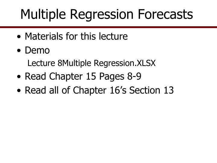
Multiple Regression Forecasts Materials for this lecture Demo Lecture 8Multiple Regression.XLSX Read Chapter 15 Pages 8-9 Read all of Chapter 16 s Section 13

Black Swans (BSs) -- Taleb BSs low probability events An outlier outside realm of reasonable expectations Carries an extreme impact Human nature causes us to concoct explanations Black swans are an example of uncertainty Uncertainty is generated by unknown probability distributions Risk is generated by known distributions 2008 recession was a BSs A depression is a BSs Dramatic increases of grain prices in 2006 and 2007 Dramatic increase in cotton price in 2010

Fat Tails and Forecasting Mandelbrot founder of fractile science observed that financial markets had fatter tails than an normal distribution implies. Taleb warns that people tend to underestimate risk, especially when armed with statistical models built on normal distributions. Posner offer this warning: We live in an information rich environment so we must seek out the right balance between human intuition and computer analysis. These cautions are offered now because we are expected to use a normal distribution to simulate residuals from a multiple regression model.

Structural Variation Variables you want to forecast are often dependent on other variables Qt. Demand = f( Own Price, Competing Price, Income, Population, Season, Tastes & Preferences, Trend, etc.) Y = a + b (Time) Structural models will explain most structural variation in a data series Even when we build structural models, the forecast is not perfect A residual remains as the unexplained portion

Structural Variation

Irregular Variation Erratic movements in time series that follow no recognizable regular pattern Random, white noise, or stochastic movements Risk is this non-systematic variability in the residuals This risk leads to Monte Carlo simulation of the risk for our probabilistic forecasts We recognize risks cannot be forecasted Incorporate risks into probabilistic forecasts Provide forecasts with confidence intervals

Multiple Regression Forecasts Structural model of the forecast variable is used when suggested by: Economic theory Knowledge of the industry Relationship to other variables Economic model is being developed Examples of forecasting: Planted acres needed by ag input businesses Demand for a product sales and processors Price of corn or cattle feedlots, grain mills, etc. Govt. payments Congressional Budget Office Exports or trade flows international ag. business

Multiple Regression Forecasts Structural model = a + b1 X1 + b2 X2 + b3 X3 + b4 X4 + e Where Xi s are exogenous variables that explain the variation of Y over the historical period Estimate parameters (a, bi s, and e) using multiple regression (or OLS) OLS is preferred because it minimizes the sum of squared residuals This is the same as reducing the risk on as much as possible, i.e., minimizing the risk for your forecast

Structural Forecast Model PltAc = f(Price , Plt , IdleAcre , X ) t t-1 t-1 t t HarvAc = f(PltAc ) t t Yield = f(Price , Yield ) t t t-1 Prod = Yield * HarvAc t t t Supply = Prod + EndStock t t t-1 Price = a + b Supply t t Domestic D = f(Price , Income / pop , Z ) t t t t Export D = f(Price , Y ) t t t End Stock = Supply - Domestic D - Export D t t t t

Steps to Build Multiple Regression Models Plot the Y variable in search of: trend, seasonal, cyclical, structural, and irregular variation Plot Y vs. each X to see the structural relationship and how X may explain Y; calculate correlation coefficients to Y Hypothesize the model equation(s) with all likely Xs to explain the Y, based on knowledge of industry & theory Wheat production forecasting model is Plt Act= f(E(Pricet), Plt Act-1, E(PthCropt), Trend, Yieldt-1) Harvested Act= a + b Plt Act Yieldt= a + b Tt Prodt= Harvested Act* Yieldt Estimate and re-estimate the model with OLS Make the deterministic forecast Make the forecast stochastic for a probabilistic forecast

US Planted Wheat Acreage Model Plt Act= f(E(Pricet), Yieldt-1, CRPt, Yearst) Statistically significant betas for Trend (years variable) and Price Leave CRP in model because of policy analysis and it has the correct sign Use Trend (years) over Yieldt-1, Trend masks the effects of Yield

Multiple Regression Forecasts Specify alternative values for X s and forecast the Deterministic Component Multiply Betas by their respective X s Forecast Acres for alternative Prices and CRP Lagged Yield and Year are constant in scenarios

Multiple Regression Forecasts Probabilistic forecast uses T+Iand (Std Dev) and assume a normal distrib. for residuals T+i= T+i+ NORM(0, ) or T+i= NORM( T+i, )

Multiple Regression Forecasts Present probabilistic forecast as a PDF with 95% Confidence Interval shown here as the bars about the mean for a probability density function (PDF)

Regression Model for Growth Some data display a growth pattern Easy to forecast with multiple regression Add T2 variable to capture the growth or decay of Y variable Growth function = a + b1T+ b2T2 Log( ) = a + b1 Log(T) Log( ) = a + b1 T See Decay Function worksheet for several examples for handling this problem Double Log Single Log

Multiple Regression Forecasts Single Log Form Log (Yt) = b0 + b1 T Double Log Form Log (Yt) = b0 + b1 Log (T)

Regression Model For Decay Functions Some data display a decay pattern Forecast them with multiple regression Add an exogenous variable to capture the growth or decay of forecast variable Decay function = a + b1(1/T) + b2(1/T2)

Forecasting Growth or Decay Patterns Here is the regression result for estimating a decay function t = a + b1 (1/Tt) or t = a + b1 (1/Tt) + b2 (1/Tt2) Observed and Predicted Values for KOV 150 100 50 0 -50 Predicted Lower 95% Predict. Interval Lower 95% Conf. Interval Observed Upper 95% Predict. Interval Upper 95% Conf. Interval

Multiple Regression Forecasts Examine a structural regression model that contains Trend and an X variable = a + b1T + b2Xt does not explain all of the variability, a seasonal or cyclical variability may be present, if so, you need to remove its effect

Goodness of Fit Measures Models with high R2 may not forecast well If add enough Xs can get high R2 T 2 e t 2 t=1 R = 1 - T 2 (Y - Y) t t=1 R-Bar2 is preferred as it is not affected by no. Xs Selecting based on highest R2 same as using minimum Mean Squared Error MSE =( et2)/T

Goodness of Fit Measures Models with high R2 may not forecast well If add enough Xs can get high R2 T 2 e t 2 t=1 R = 1 - T 2 (Y - Y) t t=1 R-Bar2 is preferred as it is not affected by no. Xs Selecting based on highest R2 same as using minimum Mean Squared Error MSE =( et2)/T

Goodness of Fit Measures I like to follow these simple rules, in this order Correct parameter signs based on sound economic theory for al variables For supply beta on price must be positive, etc. Student t ratios greater than 2.0 and/or P values for betas less than 0.05 F ratio larger than 20.0 R2 as large as you can get MAPE (mean absolute percent error) less than 0.1 (or 10%) For large models OLS is preferred

Goodness of Fit Measures Akaike Information Criterion (AIC) T AIC = exp (2k Schwarz Information Criterion (SIC) 3.5 3.5 2 T) ( e / T) t SIC SIC 3.0 3.0 t=1 2.5 2.5 Penalty Factor Penalty Factor 2.0 2.0 T AIC AIC SIC = T (k 2 1.5 1.5 T) ( e / T) t s2 s2 1.0 1.0 t=1 0.5 0.5 For T = 100 and k goes from 1 to 25 .05 .05 .10 .10 .15 .15 .20 .20 .25 .25 k/T k/T The SIC affords the greatest penalty for just adding Xs. The AIC is second best and the R2 would be the poorest.

Goodness of Fit Measures Summary of goodness of fit measures SIC, AIC, and S2 are sensitive to both k and T The S2 is small and rises slowly as k/T increases AIC and SIC rise faster as k/T increases SIC is most sensitive to k/T increases

Goodness of Fit Measures MSE works best to determine best model for in sample forecasting R2 does not penalize for adding k s R-Bar2 is based on S2 so it provides some penalty as k increases AIC is better then R2 but SIC results in the most parsimonious models (fewest k s) R2