Multipole Analysis of Electromagnetic

Front ends encompass key components such as HTML, CSS, JS, and DOM, with challenges in usability, compatibility, performance, and accessibility. Design concepts emphasize separation of style, minimizing user memory load, and semantic markup, evolving since the 1990s. Understanding the DOM structure, tags, attributes, and the interaction between client and server are essential. The growth and complexities of web development present both opportunities and challenges, shaping the online experience."

Download Presentation

Please find below an Image/Link to download the presentation.
The content on the website is provided AS IS for your information and personal use only. It may not be sold, licensed, or shared on other websites without obtaining consent from the author.If you encounter any issues during the download, it is possible that the publisher has removed the file from their server.
You are allowed to download the files provided on this website for personal or commercial use, subject to the condition that they are used lawfully. All files are the property of their respective owners.
The content on the website is provided AS IS for your information and personal use only. It may not be sold, licensed, or shared on other websites without obtaining consent from the author.
E N D
Presentation Transcript
Multipole Analysis of Electromagnetic Scattering COMSOL
Multipole Expansion The field scattered by a particle, regardless of the particle s geometrical shape or composition, can always be expressed through the multipole expansion. The expression for the electric field reads (see Ref. 1): The vector functions
Multipole Expansion and generate a complete basis, where each function describes the field created by a unique multipole.
Multipole Coefficients The coefficients aE(l,m) and aM(l,m) characterize the scatterer as they reveal the electric and magnetic excitations in it. The integer ldescribes the order of the multipole (dipole, quadrupole, ), whereas the subscripts E and M distinguish between electric and magnetic multipoles. The integer m describes the amount of the z-component of angular momentum that is carried per photon.
Multipole Coefficients For optical scatterers, the source of the scattered field is the scattering current density where h is the permittivity of the host medium and E(r) is the total field. The multipole coefficients can be extracted from the scattering current density, using volume integrals over the whole space (see Ref. 2).
Mie Scattering Scattering of a plane wave by a spherical particle. Analytical solution exists as an expansion, in which the coefficients are called Mie coefficients. MATLAB code (see Ref. 3) exists for computing the Mie coefficients ( l and l). The Mie expansion is a special case of the Multipole expansion, obtained by setting all coefficients to zero, if not |m| = 1 aE(l,-1) = -aE(l,1) aM(l,-1) = aM(l,1) Connection between the remaining multipole coefficients and the Mie coefficients is aE(l,1) = - l aM(l,1) = - l
COMSOL Implementation Equations for extracting aE(l,1) and aM(l,1) are implemented in COMSOL using functions and variables Implementation can be added to any scattering model Also applicable to periodic systems
Associated Legendre Polynomials Rodrigues' formula is used for calculating the associated Legendre polynomials Plm(cos )
Associated Legendre Polynomials Associated Legendre Polynomial
Angular Functions Function tau
Angular Functions Function pi
Coefficient O Coefficient O
Multipole Variables Calculation of aE(l,1) and aM(l,1) Defined under Component 1 > Definitions
Mie Benchmark Mie scattering as a benchmark 600 nm vacuum wavelength Au sphere of 100 nm radius Host medium with a refractive index of 1.5 Numerical results are compared to Mie coefficients evaluated in MATLAB Note: COMSOL uses exp(+j t) convention, which is handled by setting the imaginary unit i j in the equations of this presentation. Complex-conjugation of obtained multipole coefficients returns to exp(-j t) convention.
Benchmark Results Electric Multipole Coefficients l m=-3, ae (1) m=-2, ae (1) m=-1, ae (1) m=0, ae (1) m=1, ae (1) m=2, ae (1) m=3, ae (1) 1 0 0 0.93538 + 0.082177i 3.8439E-5 + 2.6268E- 5i -0.93537 - 0.082191i 0 0 2 0 -4.4753E-5 - 7.4743E- 6i 0.70154 + 0.21893i -8.3438E-6 + 4.0457E- 5i -0.70154 - 0.21893i 2.3403E-5 + 3.7582E- 5i 0 3 -5.2441E-6 - 9.8016E- 6i -1.9776E-5 - 7.0469E- 6i 0.0075631 + 0.038522i -1.74E-6 - 2.6072E-6i -0.0075571 - 0.038524i 1.804E-5 - 6.096E-6i -1.3288E-5 + 5.1912E- 6i
Benchmark Results Magnetic Multipole Coefficients l m=-3, am (1) m=-2, am (1) m=-1, am (1) m=0, am (1) m=1, am (1) m=2, am (1) m=3, am (1) 1 0 0 -0.094182 + 0.26713i 1.3235E-6 + 1.2755E- 6i -0.094186 + 0.26714i 0 0 2 0 5.0097E-7 + 4.0868E- 7i -0.0037616 + 0.034094i 2.9986E-6 + 4.3089E- 7i -0.0037614 + 0.034094i 1.4535E-6 - 1.4479E- 6i 0 3 -2.1472E-7 + 9.8539E- 8i -8.4862E-8 - 2.0176E- 7i -1.7064E-4 + 0.001774i -2.7469E-8 - 2.8486E- 7i -1.7058E-4 + 0.0017741i 9.7061E-8 - 1.446E-7i 3.4911E-7 - 3.5377E- 7i
Comparison to Reference Values Conjugate and negate the values in the m = 1 column to get values according to the exp(- j t) convention
Comparison to Reference Values Mie Coefficients l m -conj(ae) (1) -conj(am) (1) 1 1 0.93537 - 0.082191i 0.094186 + 0.26714i 2 1 0.70154 - 0.21893i 0.0037614 + 0.034094i 3 1 0.0075571 - 0.038524i 1.7058E-4 + 0.0017741i
Reference Values Reference Values, using exp(-j t) convention Reference Values l alpha_l beta_l 1 0.9350 - 0.0826i 0.0941 + 0.2671i 2 0.7003 - 0.2209i 0.0038 + 0.0341i 3 0.0075 - 0.0384i 0.0002 + 0.0018i COMSOL values and reference values agree well
Cross Sections Scattering cross setion: Extinction cross setion:
Cross Sections Interaction Cross Sections Integral: Scattering cross section (m^2) Integral: Absorption cross section (m^2) Integral: Extinction cross section (m^2) 1.4268E-13 2.7156E-14 1.6983E-13
Cross Sections Cross Sections from Fields lambda0 ( m) Scattering cross section (m^2) Absorption cross section (m^2) Extinction cross section (m^2) 0.6 1.4201E-13 2.7199E-14 1.6921E-13 Cross sections from MATLAB code Cross Section (m2) Value Scattering 1.4252e-13 Absorption 2.7148e-14 Extinction 1.6967e-13
Modal Scattering Cross Section Only essential contributions from m = -1 and m = 1 terms.
References 1. J. D. Jackson, Classical Electrodynamics, 3rd Ed., Wiley, 1999. 2. P. Grahn, A. Shevchenko, and M. Kaivola, "Electromagnetic multipole theory for optical nanomaterials," New Journal of Physics, vol. 14, no. 9, p. 093033, 2012. 3. C. M tzler, "MATLAB functions for Mie scattering and absorption, version 2," in IAP Research Report, University of Bern, 2002.