Learn about network flows and their applications in business logistics and revenue management, including solving the shortest path problem using linear programs. Explore examples such as routing, scheduling, assignment, warehouse planning, and supply chains. Understand the concept of cost of edges in a directed graph and how to find the shortest path from s to t. Dive into linear programming and decision variables for path calculations.
Please find below an Image/Link to download the presentation.
The content on the website is provided AS IS for your information and personal use only. It may not be sold, licensed, or shared on other websites without obtaining consent from the author. If you encounter any issues during the download, it is possible that the publisher has removed the file from their server.
You are allowed to download the files provided on this website for personal or commercial use, subject to the condition that they are used lawfully. All files are the property of their respective owners.
The content on the website is provided AS IS for your information and personal use only. It may not be sold, licensed, or shared on other websites without obtaining consent from the author.
Roadmap for Rest of the Class Next and Final Applied Module: Business Logistics and Revenue Management Need our last technique: Network Flows (today) Revisit Basic Feasible Solutions Example Problems Routing Scheduling Assignment Warehouse planning Supply Chains Pricing and Revenue Management Budgeted Advertising (revisit duality) Revisit Each module with one advanced example
Shortest Path Problem Find the shortest path from s to t Using linear programs Many direct applications Web applications to compute routes Indirect applications Currency arbitrage Most reliable path Beautiful structure: BFSs, duality Generalizes to Min-cost Flows
Notation Given a directed graph G V = Set of nodes in the graph, eg. {s, p, q, r, t} N = Number of nodes, eg. N = 5 p 6 4 t 2 s 3 1 2 4 r q
Notation Given a directed graph G E = Set of edges, eg. {(s,p), (p,s), (s,q), (q,s),(p,t), (q,r), (r,t)} M = Number of edges, eg. M = 7 p 6 4 t 2 s 3 1 2 4 r q
Notation Given a directed graph G c(u,v) = Cost of edge from u to v, eg. c(s,p) = 4, whereas c(s,t) is undefined p 6 4 t 2 s 3 1 2 4 r q
Notation Given a directed graph G Assume that s is the start and t the terminating point of the path we want to find p 6 4 t 2 s 3 1 2 4 r q
Notation Given a directed graph G Assume that s is the start and t the terminating point of the path we want to find p 6 4 G, V, E, N, M, c, s, t are all just a convention; we will use other symbols where necessary t 2 s 3 1 2 4 r q
Linear Program? Decision Variables? A variable for every path? Number of s-t paths in this graph = 70 t Number of s-t paths in 10 X 10 grid = 184,756 In 20 X 20 grid = 137,846,528,820 s
Linear Program? Decision Variables? A variable for every edge x(u,v): The amount of edge (u,v) used in the path, perhaps fractionally x(u,v) = 1 : The edge is used on the path x(u,v) = 0 : The edge is not used x(u,v) = : The edge is used half the time x(u,v): Leave u, enter v
Constraints x(u,v) 0 x(u,v) 1 If you enter a vertex other than s or t, you must leave it You must leave s once You must enter t once
Constraints x(u,v) 0 x(u,v) 1 If you enter a vertex other than s or t, you must leave it exactly as much as you enter it You must leave s once more than you enter it You must enter t once more than you leave it
Solution for Example x(s,q) = x(q,r) = x(r,t) = 1; all other x s are 0 p 6 4 t 2 s 3 1 2 4 r q
Minimum Cost Flow (MCF) Need to ship some good from supply nodes to demand nodes over a network Example: the good could be crude oil; the network could be a network of pipelines; the supply nodes could be oil fields; the demand nodes could be refineries Assumption: The good is divisible, so we can ship fractional amounts of a good over an edge Fundamental problem: generalizes shortest paths; maximum compatibility matching; max- flow
Modeling the Network The network is modeled as a directed graph G V = Set of nodes; E = Set of edges N = number of nodes; M = number of edges c(v,w) = cost of edge (v,w) u(v,w) = capacity of edge (v,w) Capacity of the edge: the maximum amount of flow on the edge
Modeling the Network The network is modeled as a directed graph G V = Set of nodes; E = Set of edges N = number of nodes; M = number of edges c(v,w) = cost of edge (v,w) u(v,w) = capacity of edge (v,w) Capacity of the edge: the maximum amount of flow on the edge
Modeling the Network The network is modeled as a directed graph G V = Set of nodes; E = Set of edges N = number of nodes; M = number of edges c(v,w) = cost of edge (v,w) u(v,w) = capacity of edge (v,w) Capacity of the edge: the maximum amount of flow on the edge
Modeling Demands Demand of a node: The amount of the good that a node wants to consume Supply of a node: The amount of the good that a node wants to produce Modeled as a single number, d(v), for node v d(v) is positive for demand nodes d(v) is negative for supply nodes d(v) = 0 otherwise
Can Demands be Arbitrary? For the problem to be feasible, should the sum of the demands be 1. Strictly Negative? 2. Zero 3. Strictly Positive? 4. Doesn t matter.
Can Demands be Arbitrary? For the problem to be feasible, should the sum of the demands be 1. Strictly Negative? 2. Zero 3. Strictly Positive? 4. Doesn t matter.
Reduction to MCF Very powerful tool Suppose we are reducing a problem P to MCF Must specify how to obtain The graph G (nodes, edges) Edge capacities u and costs c Node demands d from the parameters of the given problem P Must specify how the solution x to MCF gives a solution to P
A Simple Reduction Reducing s-t Shortest Paths to MCF Use the same graph G and the given costs c Set d(s) = -1, d(t) = 1, d(v) = 0 for all other nodes Set u(v,w) = 1 for all edges (v,w) (Or, set u(v,w) = for all edges (v,w)) The solution x(v,w) to the MCF is also a solution to the shortest path problem Hence, MCF is more general than shortest paths
A Simple Example Every edge has a cost and a capacity, written as (c, u) p (6,1) (4,1) t (2,1) s (3,1) (1,1) (2,1) (4,1) r q
A Simple Example Every node has a demand d = 0 p (6,1) (4,1) t d = 1 (2,1) s d = -1 (3,1) (1,1) (2,1) (4,1) r q d = 0 d = 0
A Simple Example Every node has a demand capacities can be d = 0 p (6, ) (4, ) t d = 1 (2, ) s d = -1 (3, ) (1, ) (2, ) (4, ) r q d = 0 d = 0
Infinite Capacities? Can handle infinite capacity edges by just removing the capacity constraint for those edges For shortest paths Setting capacity = guarantees that there will never be an optimum solution if there is a negative cost cycle (better fits the spirit of the problem) Setting capacity = 1 guarantees that there will be an optimum solution if there is a feasible solution
Next Steps Theory: Examine Basic Feasible Solutions Reductions: See two more examples Hands On: Solve an example problem Illustrate capacity constraints A nice trick for generating the constraint matrix A
Main Theorem For an instance of a Minimum Cost Flow Problem, if (a) Every demand is integral and (b) Every capacity is integral then Every Basic Feasible Solution is Integral Very useful, since in many applications (eg. Shortest paths), fractional solutions do not make sense
Proof Sketch 1. Start with any feasible fractional solution 2. Find a cycle of edges (ignoring directions) such that every edge on the cycle has fractional flow 3. Show that along this cycle, flow can be increased a little clockwise, as well as counterclockwise The original fractional solution was an average of two other feasible solutions, and hence not a BFS
A Simple Example Labels on edges are (costs, capacities) d = 0 p (6,1) (4,1) t d = 1 (2,1) s d = -1 (3,1) (1,1) (2,1) (4,1) r q d = 0 d = 0
Step 2: Find a Cycle of Fractionally Used Edges Labels on edges are flows Start with an arbitrary fractional edge d = 0 p 0.6 0.6 t d = 1 0 s d = -1 0.4 0.4 0.4 0 r q d = 0 d = 0
Step 2: Find a Cycle of Fractionally Used Edges Labels on edges are flows Start with an arbitrary fractional edge d = 0 p 0.6 0.6 t d = 1 0 s d = -1 0.4 0.4 0.4 0 r q d = 0 d = 0
Step 2: Find a Cycle of Fractionally Used Edges Since t has integer demand, there must be another edge incident on t with fractional flow Labels on edges are flows d = 0 p 0.6 0.6 t d = 1 0 s d = -1 0.4 0.4 0.4 0 r q d = 0 d = 0
Step 2: Find a Cycle of Fractionally Used Edges Since t has integer demand, there must be another edge incident on t with fractional flow Labels on edges are flows d = 0 p 0.6 0.6 t d = 1 0 s d = -1 0.4 0.4 0.4 0 r q d = 0 d = 0
Step 2: Find a Cycle of Fractionally Used Edges Use the same argument at r Labels on edges are flows d = 0 p 0.6 0.6 t d = 1 0 s d = -1 0.4 0.4 0.4 0 r q d = 0 d = 0
Step 2: Find a Cycle of Fractionally Used Edges Use the same argument at r Labels on edges are flows d = 0 p 0.6 0.6 t d = 1 0 s d = -1 0.4 0.4 0.4 0 r q d = 0 d = 0
Step 2: Find a Cycle of Fractionally Used Edges Use the same argument at q Labels on edges are flows d = 0 p 0.6 0.6 t d = 1 0 s d = -1 0.4 0.4 0.4 0 r q d = 0 d = 0
Step 2: Find a Cycle of Fractionally Used Edges Use the same argument at q Labels on edges are flows d = 0 p 0.6 0.6 t d = 1 0 s d = -1 0.4 0.4 0.4 0 r q d = 0 d = 0
Step 2: Find a Cycle of Fractionally Used Edges Use the same argument at s Labels on edges are flows d = 0 p 0.6 0.6 t d = 1 0 s d = -1 0.4 0.4 0.4 0 r q d = 0 d = 0
Step 2: Find a Cycle of Fractionally Used Edges Use the same argument at s Labels on edges are flows d = 0 p 0.6 0.6 t d = 1 0 s d = -1 0.4 0.4 0.4 0 r q d = 0 d = 0
Step 2: Find a Cycle of Fractionally Used Edges We have our cycle Labels on edges are flows d = 0 p 0.6 0.6 t d = 1 0 s d = -1 0.4 0.4 0.4 0 r q d = 0 d = 0
Step 2: Find a Cycle of Fractionally Used Edges We have our cycle Labels on edges are flows d = 0 p 0.6 0.6 t d = 1 0 s d = -1 0.4 Strongly used the fact that demands are integer 0.4 0.4 0 r q d = 0 d = 0
Step 3: Find Two New Feasible Solutions None of the edges on the cycle is at capacity Labels on edges are flows d = 0 p 0.6 0.6 t d = 1 0 s d = -1 0.4 0.4 0.4 0 r q d = 0 d = 0
Step 3: Find Two New Feasible Solutions None of the edges on the cycle is at capacity Labels on edges are flows d = 0 p 0.6 0.6 t d = 1 0 s d = -1 0.4 Strongly used the fact that capacities are integer 0.4 0.4 0 r q d = 0 d = 0


")