Neural Networks: Overview and Feedforward Networks in Pattern Recognition

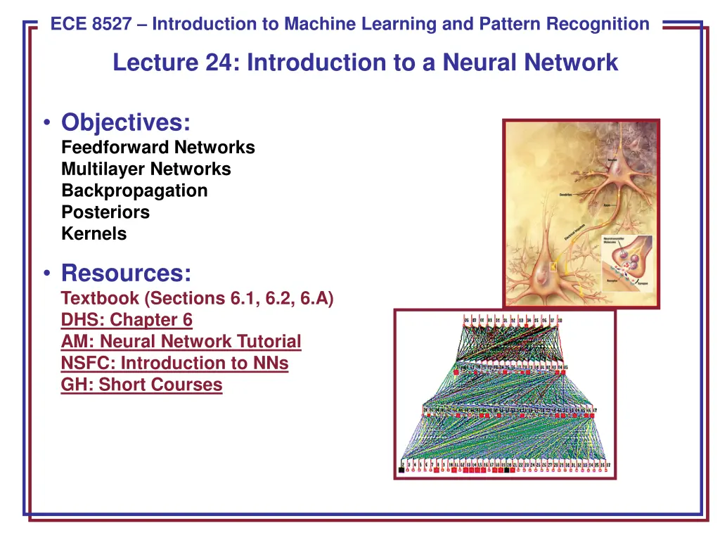
ECE 8443 Pattern Recognition ECE 8527 Introduction to Machine Learning and Pattern Recognition Lecture 24: Introduction to a Neural Network Objectives: Feedforward Networks Multilayer Networks Backpropagation Posteriors Kernels Resources: Textbook (Sections 6.1, 6.2, 6.A) DHS: Chapter 6 AM: Neural Network Tutorial NSFC: Introduction to NNs GH: Short Courses

Overview There are many problems for which linear discriminant functions are insufficient for minimum error. Previous methods, such as Support Vector Machines require judicious choice of a kernel function (though data-driven methods to estimate kernels exist). A brute approach might be to select a complete basis set such as all polynomials; such a classifier would require too many parameters to be determined from a limited number of training samples. There is no automatic method for determining the nonlinearities when no information is provided to the classifier. Multilayer Neural Networks attempt to learn the form of the nonlinearity from the training data. These were loosely motivated by attempts to emulate behavior of the human brain, though the individual computation units (e.g., a node) and training procedures (e.g., backpropagation) are not intended to replicate properties of a human brain. Learning algorithms are generally gradient-descent approaches to minimizing error. ECE 8527: Lecture 24, Slide 1

Feedforward Networks A three-layer neural network consists of an input layer, a hidden layer and an output layer interconnected by modifiable weights represented by links between layers. A bias term that is connected to all units. This simple network can solve the exclusive-OR problem. The hidden and output units from the linear weighted sum of their inputs and perform a simple thresholding (+1 if the inputs are greater than zero, -1 otherwise). ECE 8527: Lecture 24, Slide 2

Definitions A single bias unit is connected to each unit other than the input units. d d wt = + = = x = i = i net x w w x w Net activation: j 0 j i ji j i ji 1 0 where the subscript i indexes units in the input layer,jin the hidden; wji denotes the input-to-hidden layer weights at the hidden unit j. Each hidden unit emits an output that is a nonlinear function of its activation: yj = f(netj) Even though the individual computational units are simple (e.g., a simple threshold), a collection of large numbers of simple nonlinear units can result in a powerful learning machine (similar to the human brain). Each output unit similarly computes its net activation based on the hidden unit signals as: n n w y w w y net 0 1 wt H H = + = = y = j = j k 0 k j kj k j kj where the subscript k indexes units in the output layer andnHdenotes the number of hidden units. zkwill represent the output for systems with more than one output node. An output unit computes zk = f(netk). ECE 8527: Lecture 24, Slide 3

Computations The hidden unit y1computes the boundary: 0 y1 = +1 x1 + x2 + 0.5 = 0 < 0 y1 = -1 The hidden unit y2 computes the boundary: 0 y2 = +1 x1 + x2 -1.5 = 0 < 0 y2 = -1 The final output unit emits z1 = +1 iff y1 = +1 and y2 = +1 zk = y1and not y2 = (x1 or x2) and not (x1 and x2) = x1 XOR x2 ECE 8527: Lecture 24, Slide 4

General Feedforward Operation For c output units: j n i d H = + + = g x ( ) k 1,..., c z f w f w x w w 0 0 k k kj ji i j k = = 1 1 Hidden units enable us to express more complicated nonlinear functions and thus extend the classification. The activation function does not have to be a sign function, it is often required to be continuous and differentiable. We can allow the activation in the output layer to be different from the activation function in the hidden layer or have different activation for each individual unit. We assume for now that all activation functions to be identical. Can every decision be implemented by a three-layer network? Yes (due to A. Kolmogorov): Any continuous function from input to output can be implemented in a three-layer net, given sufficient number of hidden units nH,proper nonlinearities, and weights. ( ) + 2 1 n n = 1 , 0 [ = = j ( ) ( ) x I ( ]; ) 2 g x x I n j ij i 1 for properly chosen functions jand ij ECE 8527: Lecture 24, Slide 5

General Feedforward Operation (Cont.) Each of the 2n+1 hidden units j takes as input a sum of d nonlinear functions, one for each input feature xi . Each hidden unit emits a nonlinear function jof its total input. The output unit emits the sum of the contributions of the hidden units. Unfortunately: Kolmogorov s theorem tells us very little about how to find the nonlinear functions based on data; this is the central problem in network- based pattern recognition. ECE 8527: Lecture 24, Slide 6

Backpropagation Any function from input to output can be implemented as a three-layer neural network. These results are of greater theoretical interest than practical, since the construction of such a network requires the nonlinear functions and the weight values which are unknown! Our goal now is to set the interconnection weights based on the training patterns and the desired outputs. In a three-layer network, it is a straightforward matter to understand how the output, and thus the error, depend on the hidden-to-output layer weights. The power of backpropagation is that it enables us to compute an effective error for each hidden unit, and thus derive a learning rule for the input-to- hidden weights, this is known as the credit assignment problem. Networks have two modes of operation: Feedforward: consists of presenting a pattern to the input units and passing (or feeding) the signals through the network in order to get outputs units. Learning: Supervised learning consists of presenting an input pattern and modifying the network parameters (weights) to reduce distances between the computed output and the desired output. ECE 8527: Lecture 24, Slide 7

Backpropagation (Cont.) ECE 8527: Lecture 24, Slide 8

Network Learning Let tk be the k-th target (or desired) output and zk be the k-th computed output with k = 1, , c and w represents all the weights of the network. 1 ) (w 1 c 2 2 = = Training error: = k ( ) J t z t z k k 2 2 1 The backpropagation learning rule is based on gradient descent: The weights are initialized with pseudo-random values and are changed in J = a direction that will reduce the error: w w where is the learning rate which indicates the relative size of the change in weights. The weight are updated using: w(m +1) = w (m) + w (m). J J net J net = = k k . Error on the hidden to-output weights: k net w w w kj k kj kj = where the sensitivity of unit k is defined as: k net k and describes how the overall error changes with the activation of the unit s net: J J z = = = k . ( ) ( ' ) t z f net k k k k net net z k k k ECE 8527: Lecture 24, Slide 9

Network Learning (Cont.) net Since netk= wkt.y: = k y j w kj Therefore, the weight update (or learning rule) for the hidden-to-output weights is: wkj = kyj = (tk zk) f (netk)yj y net J J j j = . . The error on the input-to-hidden units is: net w y w ji j j ji y 1 J z c c 2 = = k = k = k ( ) ( ) t z t z The first term is given by: k k k k 2 y y 1 1 j j j net z net c c = = k k = k = k ( ) . ( ) ( ' ) t z t z f net w k k k k k kj y 1 1 k j c = k ( ' ) f net w 1 We define the sensitivity for a hidden unit: j j kj k which demonstrates that the sensitivity at a hidden unit is simply the sum of the individual sensitivities at the output units weighted by the hidden-to- output weights wkj; all multipled by f (netj). The learning rule for the input-to-hidden weights is: = = ( ' ) w x w f net x ji i j kj k j i j ECE 8527: Lecture 24, Slide 10

Stochastic Back Propagation Starting with a pseudo-random weight configuration, the stochastic backpropagation algorithm can be written as: Begin initialize nH; w, criterion , , m 0 do m m + 1 xm randomly chosen pattern wji wji + jxi; wkj wkj + kyj until || J(w)|| < return w End ECE 8527: Lecture 24, Slide 11

Stopping Criterion One example of a stopping algorithm is to terminate the algorithm when the change in the criterion function J(w) is smaller than some preset value . There are other stopping criteria that lead to better performance than this one. Most gradient descent approaches can be applied. So far, we have considered the error on a single pattern, but we want to consider an error defined over the entirety of patterns in the training set. The total training error is the sum over the errors of n = = p n individual patterns: J J p 1 A weight update may reduce the error on the single pattern being presented but can increase the error on the full training set. However, given a large number of such individual updates, the total error decreases. ECE 8527: Lecture 24, Slide 12

Learning Curves Before training starts, the error on the training set is high; through the learning process, the error becomes smaller. The error per pattern depends on the amount of training data and the expressive power (such as the number of weights) in the network. The average error on an independent test set is always higher than on the training set, and it can decrease as well as increase. A validation set is used in order to decide when to stop training; we do not want to overfit the network and decrease the power of the classifier generalization. ECE 8527: Lecture 24, Slide 13

Gradient descent pick a starting point (w) repeat until loss doesn t decrease in all dimensions: pick a dimension move a small amount in that dimension towards decreasing loss (using the derivative) n wj= wj+h yixijexp(-yi(w xi+b)) i=1 What is this doing?

Perceptron learning algorithm! repeat until convergence (or for some # of iterations): for each training example (f1, f2, , fm, label): prediction=b+ j=1 m wjfj if prediction * label 0: // they don t agree for each wj: wj = wj + fj*label b = b + label wj=wj+hyixijexp(-yi(w xi+b)) or where c=hexp(-yi(w xi+b)) wj=wj+xijyic

The constant c=hexp(-yi(w xi+b)) prediction label learning rate When is this large/small?

The constant c=hexp(-yi(w xi+b)) prediction label If they re the same sign, as the predicted gets larger there update gets smaller If they re different, the more different they are, the bigger the update

One concern n exp(-yi(w xi+b)) argminw,b i=1 loss What is this calculated on? Is this what we want to optimize? w

Perceptron learning algorithm! repeat until convergence (or for some # of iterations): for each training example (f1, f2, , fm, label): prediction=b+ j=1 m wjfj if prediction * label 0: // they don t agree for each wj: wj = wj + fj*label b = b + label Note: for gradient descent, we always update wj=wj+hyixijexp(-yi(w xi+b)) or where c=hexp(-yi(w xi+b)) wj=wj+xijyic

One concern n exp(-yi(w xi+b)) argminw,b i=1 loss We re calculating this on the training set We still need to be careful about overfitting! w The min w,b on the training set is generally NOT the min for the test set How did we deal with this for the perceptron algorithm?

Overfitting revisited: regularization A regularizer is an additional criteria to the loss function to make sure that we don t overfit It s called a regularizer since it tries to keep the parameters more normal/regular It is a bias on the model forces the learning to prefer certain types of weights over others n loss(yy')+lregularizer(w,b) argminw,b i=1

Regularizers n 0=b+ wjfj j=1 Should we allow all possible weights? Any preferences? What makes for a simpler model for a linear model?

Regularizers n 0=b+ wjfj j=1 Generally, we don t want huge weights If weights are large, a small change in a feature can result in a large change in the prediction Also gives too much weight to any one feature Might also prefer weights of 0 for features that aren t useful How do we encourage small weights? or penalize large weights?

Regularizers n 0=b+ wjfj j=1 How do we encourage small weights? or penalize large weights? n loss(yy')+lregularizer(w,b) argminw,b i=1

Common regularizers wj r(w,b)= wj sum of the weights wj 2 r(w,b)= wj sum of the squared weights What s the difference between these?

Summary Introduced the concept of a feedforward neural network. Described the basic computational structure. Described how to train this network using backpropagation. Discussed stopping criterion. Described the problems associated with learning, notably overfitting. What we didn t discuss: Many, many forms of neural networks. Three historically important types of networks to consider: ( ) = = j 0 n H x z w Basis functions: k kj j Boltzmann machines: a type of simulated annealing stochastic recurrent neural network. Recurrent networks: used extensively in time series analysis. Posterior estimation: in the limit of infinite data the outputs approximate a true a posteriori probability in the least squares sense. Alternative training strategies and learning rules. ECE 8527: Lecture 24, Slide 26