New Developments in Attachment Theory" (45 characters)
Attachment theory is a key aspect of social work theory and education, with ongoing debates and politicization surrounding its relevance. This presentation delves into practitioners' reflections on attachment, highlighting the importance and challenges they face in applying contemporary attachment research findings. Researchers identify crucial ideas to support social workers in enhancing their understanding and practice in this area, aiming to bridge the gap between outdated perceptions and current knowledge. The discussion invites participation and feedback from professionals interested in exploring attachment theory within the context of social work. Contact Dr. Sarah Foster for more information and to contribute insights to this evolving discourse. (500 characters)

Download Presentation

Please find below an Image/Link to download the presentation.
The content on the website is provided AS IS for your information and personal use only. It may not be sold, licensed, or shared on other websites without obtaining consent from the author.If you encounter any issues during the download, it is possible that the publisher has removed the file from their server.
You are allowed to download the files provided on this website for personal or commercial use, subject to the condition that they are used lawfully. All files are the property of their respective owners.
The content on the website is provided AS IS for your information and personal use only. It may not be sold, licensed, or shared on other websites without obtaining consent from the author.
E N D
Presentation Transcript
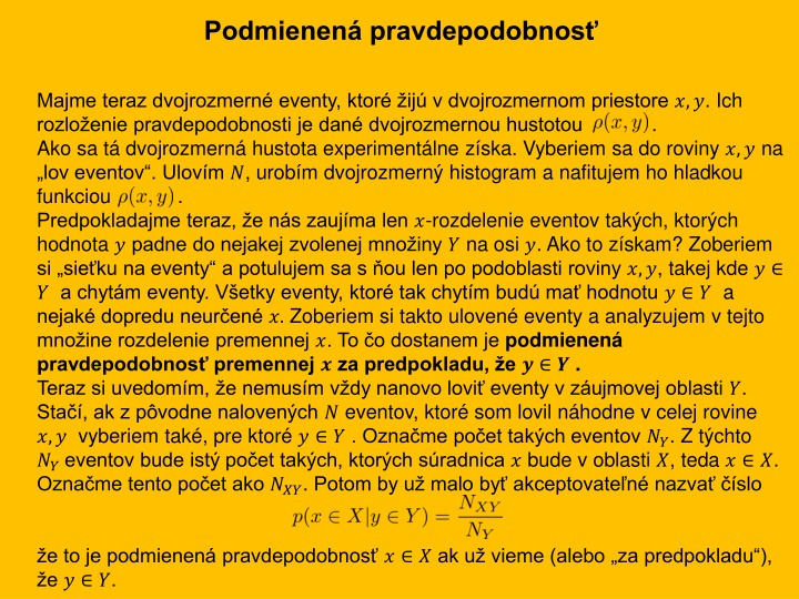
Podmienen pravdepodobnos Majme teraz dvojrozmern eventy, ktor ij v dvojrozmernom priestore ?,?. Ich rozlo enie pravdepodobnosti je dan dvojrozmernou hustotou . Ako sa t dvojrozmern hustota experiment lne z ska. Vyberiem sa do roviny ?,? na lov eventov . Ulov m ?, urob m dvojrozmern histogram a nafitujem ho hladkou funkciou . Predpokladajme teraz, e n s zauj ma len ?-rozdelenie eventov tak ch, ktor ch hodnota ?padne do nejakej zvolenej mno iny ? na osi ?. Ako to z skam? Zoberiem si sie ku na eventy a potulujem sa s ou len po podoblasti roviny ?,?, takej kde ? ?a chyt m eventy. V etky eventy, ktor tak chyt m bud ma hodnotu ? ? a nejak dopredu neur en ?. Zoberiem si takto uloven eventy a analyzujem v tejto mno ine rozdelenie premennej ?. To o dostanem je podmienen pravdepodobnos premennej ?za predpokladu, e ? ? . Teraz si uvedom m, e nemus m v dy nanovo lovi eventy v z ujmovej oblasti ?. Sta , ak z p vodne naloven ch ? eventov, ktor som lovil n hodne v celej rovine ?,? vyberiem tak , pre ktor ? ?. Ozna me po et tak ch eventov ??. Z t chto ??eventov bude ist po et tak ch, ktor ch s radnica ? bude v oblasti ?, teda ? ?. Ozna me tento po et ako ???. Potom by u malo by akceptovate n nazva slo e to je podmienen pravdepodobnos ? ?ak u vieme (alebo za predpokladu ), e ? ?.
Podmienen pravdepodobnos Vypo tame teraz ??,???. Ak v etk ch pokusov je ?, potom z nich tak ch, kde ? ? je zrejme Z t chto eventov sme potom vyberali tak , kde s asne bolo aj ? ?. Ich po et sme ozna ili ???. Uvedomme si ale, e tie eventy nemus me vybera z t ch ?? eventov, rovnak eventy dostaneme ak ich budeme vybera rovno zo v etk ch ? eventov, ak budeme vybera eventy pre ktor ? ?a s asne ? ?. Bude ich Potom pre podmienen pravdepodobnos , ktor sme (d fam e s pln m pochopen m) definovali ako dostaneme a to je presne ten vzorec, ktor sa n m mo no zdal m lo pochopite n m
Continuous random events: more dimensions Independent variables Variable ? is independent of ? if the conditional probability does not depend on ? for any ?. It means that knowing information about ? does not change our expectation about ?. We shall prove that ? is independent of ? if and only if the two dimensional probability density factorizes, that is if it can be written as where on the right side we have the marginal distributions. First we prove the sufficient condition. Suppose ?(?,?) factorizes. Then and the result obviously does not depend on ?. 3
Continuous random events: more dimensions Independent variables Now we prove the necessary condition. Let us choose the regions ?,? to be very small intervals around specific (but arbitrary) values ?0,?0. Let us denote those small intervals as ??0,??0. We get Since the conditional probability is independent of ?, we can write Comparing the two results, we get since the values ?0,?0are arbitrary, we have proven the factorization. 4
Continuous random events: more dimensions Mean values We have two random variables ?,? with probability density ?(?,?). Then the following is true in general Proof: We have two independent random variables ?,? with probability density Then the following is true 5
Continuous random events: more dimensions Mean values Proof: for independent variables and we get Note: if holds, it does not necessarily mean that the variables are independent, even if it often considered as a strong hint for independence. 6
Continuous random events: no bias distribution counterexample Consider the following problem. A thin long rigid rod is randomly thrown onto a circle and intersect the circle in two points A,B forming a chord (segment AB). Denote the length of the chord as ?. Find the probability density for the random variable ?. Solution 1: Without loss of generality we can assume that all the thrown rods are parallel, perpendicular to the dash-dotted line in the figure. So the random event is fully specified by the size of the segment SB denoted as ?. Using non- biased uniform distribution of ? ?,? we get 7
Continuous random events: no bias distribution counterexample Consider the following problem. A thin long rigid rod is randomly thrown onto a circle and intersect the circle in two points A,B forming a chord (segment AB). Denote the length of the chord as ?. Find the probability density for the random variable ?. Solution 2: Without loss of generality we can assume that all the thrown rods intersect the circle in the specific point A. So the random event is fully specified by the angle ASB denoted as . Using non-biased uniform distribution of (0,2?) we get So two equally plausible solutions , two different results! 8
Random walk in one dimension: Drunken sailor Consider one-dimensional world, a line with a coordinate denoted by ?. In the point ? = 0 there is a pub. At time ? = 0 (we use discrete time) a sailor gets out of the pub and starts to make random steps of equal size but random direction (with equal probability either to the left or to the right). Suppose that after making ? steps he has got into the point with the coordinate ??. Then after making the next step he would be in the point The equation describes the dynamics of what is called a random process. If we observe one sailor during his motion, we observe one particular realization of the random process. This means, that for this particular realization in each time step a particular sign (plus or minus) is randomly chosen (for example by tossing a coin) and a particular position history is realized. Observing another sailor, the random choices in each time step would be different and we get a different realization of the random process. Each realization is described by the same dynamical equation as presented above. 10
Random walk in one dimension: Drunken sailor In the figure, there are 8 different realizations of the drunken sailor random process denoted by different colors. The plot shows the current position on the line (vertical axis) versus the time steps (horizontal axis). 11
Random walk in one dimension: Drunken sailor We have observed in the figure that with increasing time (number of steps) there is a tendency that the sailors typically get to increasing distances from the origin. Very often our primary interest is just one realization of the random process (one drunken sailor) and we would like to understand how his distance from the origin changes in time. We, of course, know, that for one sailor his particular distance from the origin is not a monotonic function of time. It might happen quite often that he would appear in the pub (at zero distance). Analyzing one particular trajectory with the aim to understand qualitatively its characteristics might be fairly complicated. Instead of that we often switch to a different problem: to understand a typical behavior within a statistical ensemble of many realizations of the same random process (as it was visualized in the figure). So we write dynamic equations for an ensemble of ? sailors performing random walk synchronously in parallel (making their n-th step in the same time instant). We get a set of equations 12
Random walk in one dimension: Drunken sailor the superscript in the parenthesis is the index denoting individual sailors in the ensemble Now we sum the equations and we get The overlines denote the average values over the ensemble, that is denotes the mean coordinate of the sailor ensemble after ? steps. For very large ? the mean step is zero, since the random signs cancel. The last recurrent equation is easily solved as 13
Random walk in one dimension: Drunken sailor This results can be qualitatively expressed as: In the mean the sailor is to be found in the pub in each time instance. The statement is almost obvious due to the left-right symmetry of the problem. However this first law of a drunken sailor does not characterize the observed fact that with increasing time the probability to find a sailor in a distance larger than something increases. To investigate this effect it is useful to square all the ensemble equations before calculating the averages. 14
Random walk in one dimension: Drunken sailor Averaging over the ensemble we get The last recurrent equation is easily solved as The second law of the drunken sailor therefore reads: Mean square of the distance of the sailor from the pub increases proportionally to the number of steps. Said alternatively the typical distance of a drunken sailor from the pub increases as the square root of the number of steps. This contrasts with the law of non-random (directional) walk : the distance (and not the square of it) increases proportionally to the number of steps. So the characterizing logo of the drunken sailor is 15
Drunken sailor application: Standard error of an arithmetic mean In mathematics and statistics, the arithmetic mean is the sum of a collection of numbers divided by the number of numbers in the collection. It is often use to decrease the measurement error of some quantity by performing the measurement several times and taking the arithmetic mean as a better estimate of the true value of the measured quantity compared to the result of a single measurement. Let the statistical error of a single measurement be (symbolically) expressed by the formula Let us make ? individual independent measurements, denoted as and calculate the arithmetic mean then the typical statistical error of the average can be estimated as 16
Drunken sailor application: Standard error of an arithmetic mean - proof Let us investigate the outcome of the i-th measurement, it differs from the true value by a random error where ??is the (individual) measurement error, usually assumed to be Gaussian- distributed with mean ? = 0 and variance ?2= 2. Then The difference between the true value and the arithmetic mean is expressed through the sum of independent individual errors this expression is the same as that giving the coordinate of a drunken sailor after ? random steps 17
Drunken sailor application: Standard error of an arithmetic mean - proof In the final formula we clearly recognize the drunken sailor ? rule . 18
Collisions in a one-dimensional world In a one-dimensional world observe a collision of two pointlike particles: one with mass ? and velocity and another with mass ? and velocity . Let us stress that we are not using vector notations here, so the velocities mean, in fact, velocity projection on the coordinate axis and as such they can be also negative. Let us denote the velocities after the collision as . It is easy to find the velocities after the collision, one gets Let us observe many particles of the type M denoted by index ? , then after ? collisions one gets Where we assume that in each collision the particle m is drawn from the same common pool of particles independently of the collision number ?. Averaging over the ensemble: In different notation: Asymptotically the initial particle velocity is completely forgotten after many collisions. 19
Squaring this equation first and only then making the ensemble average we get: Asymptotically we get The meaning oft the asymptotic solution is better understood, after we rewrite it as We can read it as Ensemble-mean kinetic energy is asymptotically the same as the mean energy of the particles from the pool. 20
Particle collisions: conclusions based on the demo A particle randomly bombarded by particles having some mean kinetic energy asymptotically forgets its initial velocity and finally reaches (mean) kinetic energy equal to the kinetic energy of the bombarding particles. The word mean here describes a statistical average within an ensemble of similar particles undergoing same random bombardments. To be more precise here we speak about kinetic energies of the translational motion. Conclusion 1: if we have an equilibrium system consisting of many types of particles (different masses) then the mean kinetic energy of all the particles will be the same. Conclusion 2: if we start with a system of different types of particles with unequal kinetic energies then after some relaxation time the mean kinetic energies of all the particles will become the same. Conclusion 3: If we have two physical systems in thermal contact (this means that they cannot exchange particles but the particles on the surface contact can collide with each other) then started from arbitrary macroscopic state the equilibrium will be reached where the mean kinetic energies of particles in the two systems will be equal 21