Non-Response in the 1958 Birth Cohort: Understanding Patterns and Implications
The study delves into non-response in the National Child Development Study (NCDS) of individuals born in England, Scotland, and Wales in 1958. It explores the types of non-response, response patterns, biases, and strategies to address attrition, aiming to maximize the plausibility of missing data assumptions. The findings shed light on the impact of attrition on sample sizes, statistical power, and result biases, underscoring the need for careful consideration of predictors of response.

Download Presentation

Please find below an Image/Link to download the presentation.
The content on the website is provided AS IS for your information and personal use only. It may not be sold, licensed, or shared on other websites without obtaining consent from the author.If you encounter any issues during the download, it is possible that the publisher has removed the file from their server.
You are allowed to download the files provided on this website for personal or commercial use, subject to the condition that they are used lawfully. All files are the property of their respective owners.
The content on the website is provided AS IS for your information and personal use only. It may not be sold, licensed, or shared on other websites without obtaining consent from the author.
E N D
Presentation Transcript
Understanding Non Response in the 1958 Birth Cohort Tarek Mostafa, Brian Dodgeon & George B. Ploubidis
Outline Introduction to the National Child Development Study (NCDS) Non-response in NCDS The three stages strategy Findings
The National Child Development Study (NCDS) The NCDS follows the lives of all people born in England, Scotland and Wales in one week of March 1958 The target sample was augmented to include immigrants born in the same week, in the first three sweeps (ages 7, 11 and 16) NCDS experienced attrition over time. Attrition is the discontinued participation of some individuals in a longitudinal survey
Non response in NCDS Types of non- response Wave 0 Wave 1 Wave 2 Wave 3 Wave 4 Wave 5 Wave 6 Wave 7 Wave 8 Wave 9 Birth 223 920 0 Age 7 Age 11 Age 16 Age 23 Age 33 Age 42 Age 46 Age 50 Age 55 1,042 410 786 1,867 1,529 542 271 0 0 0 80 797 1,151 1,160 1,776 Non-contact Not issued Refusal Other unproductive Not issued - emigrant Not issued - dead Ineligible Total 1,832 1,415 1,148 612 4,248 1,448 835 3,553 1,214 664 4,698 582 0 173 202 295 838 1,399 263 109 332 491 0 475 701 799 1,196 1,335 1,268 1,272 1,293 1,287 0 0 821 0 3,133 840 0 3,221 873 0 3,904 960 0 6,021 1,050 0 7,089 1,200 13 7,139 1,324 11 9,024 1,460 81 8,768 1,503 0 9,225 1,143
Monotone vs. Non-monotone response Response patterns Freq. Percent Monotone 5688 30.64 Non-monotone 8329 44.89 All waves 4,541 24.47 Total 18558 100
Non-response bias - implications Missing data: 1- Smaller samples, fewer transitions, incomplete histories. Loss of statistical power due to smaller samples 2- Biases in results: Disproportionate to some groups (mobile, disadvantaged, men, long working hours)
What can we do about attrition? All principled methods rely on the MAR assumption and on the correct identification of predictors of response => maximise the plausibility of MAR So far selection is arbitrary Mainly birth characteristics, reflecting economic and social circumstances: SES, housing tenure, accommodation type, London vs. rest of the country Selection of predictors matters more for studies with more waves (more missing data)
Missing data strategy Identify predictors of response at each wave of NCDS: Variables from each wave can only predict response on subsequent waves Thousands of variables are available => selection is done in three stages Pre selection: We exclude routed variables. We exclude dead respondents from each wave natural evolution of the sample Analysis: Stage 1: univariable regressions within wave Stage 2: multivariable regressions within wave Stage 3: multivariable regressions across waves
Stage 1: Univariable regressions Predictors: waves 0 to 8 (including biomedical) Response outcomes: waves 1 to 9 (including biomedical) Univariable logistic regressions (one predictor at a time) to predict response in subsequent waves Analytical sample=non-missing W0 predictors. N=15,150 N of predictors W0 Birth 19 W1 Age 7 50 W2 W3 W4 W5 W6 Biomed W7 W8 Age 11 Age 16 Age 23 Age 33 Age 42 Age 45 Age 46 Age 50 48 58 73 100 Stage 1 (input) 276 81 155 194 N of regressions for: (wave0= 19*10); (wave5=100*5); The process is automated Retained predictors with a significant impact on response at p<0.01
Stage 2: Multivariable regressions within wave. N of predictors W0 W1 W2 Birth Age 7 Age 11 Age 16 Age 23 Age 33 Age 42 Age 45 Age 46 Age 50 Stage 1 (input) 19 50 48 58 Stage 2 (input) 11 36 34 47 W3 W4 W5 W6 Biomed W7 W8 73 50 100 68 276 114 81 39 155 53 194 120 N of predictors is reduced after stage 1 Stage 2 consists of multivariable regressions using all predictors from same wave (i.e. 11 for W0, 36 for W1, 120 for W8) that were retained after Stage 1 Variables compete against each other within wave Using log binomial models (since outcome not always rare) Retain variables significant at p<0.05 This results in different subsets of predictors from each wave depending on the response outcome
Stage 3: Multivariable regressions across waves. N of predictors W0 Birth 19 11 W1 Age 7 50 36 W2 W3 W4 W5 W6 Biomed W7 W8 Age 11 Age 16 Age 23 Age 33 Age 42 Age 45 Age 46 Age 50 48 58 73 100 34 47 50 68 Stage 1 (input) Stage 2 (input) 276 114 81 39 155 53 194 120 Variables entering stage 3: N of predictors Resp 1 Resp 2 Resp 3 Resp 4 Resp 5 Resp 6 Biomed Resp 7 Resp 8 Resp 9 Age 7 Age 11 Age 16 Age 23 Age 33 Age 42 Stage 3 (input) 4 13 23 36 Age 45 Age 46 Age 50 Age 55 81 86 52 54 88 116 At this stage we let predictors from different waves compete against each other (e.g. subset of predictors from W0 and W1 predict response in W2; subset of predictors from W0, 1, 2, 3, 4 predict response in W5, ) Challenge: predictors from different waves => different levels of missingness (due to non-response over time). Predictors from earlier waves are more complete
Stage 3: Multivariable regressions across waves (continued). Solution: progressive imputation and alternation of MI and response modelling We impute missing predictors then estimate response models and so on for each wave Example W2 MI with chained equations and response modelling with log binomial models. => Set of predictors of response in each wave (sig at p<0.05). For each response outcome, the predictors can include variables from any previous wave
Results from stage 3 The number of predictors of response at each wave is reduced N of predictors Resp 1 Resp 2 Resp 3 Resp 4 Resp 5 Resp 6 Biomed Resp 7 Resp 8 Resp 9 Age 7 Age 11 Age 16 Age 23 Age 33 Age 42 Age 45 Age 46 Age 50 Age 55 4 13 23 36 52 4 9 11 17 24 Stage 3: input Stage 3: output 54 18 81 40 86 34 88 35 116 39 Predictors include all types of variables: Social, economic, health, and survey related (cooperation with sub-studies)
Examples of predictors for Wave 3 (age 16) Smoking prior to pregnancy (wave 0, birth) Physical exercise problems (balance etc) (wave 2, age 11) Social class of mother's husband (wave 0, birth) Outpatient Clinic attendances (wave 1, age 7) Number of kids aged under 21 in household, including those living away from home (wave 1, age 7)
Examples of predictors for Wave 5 (age 33) Age at birth of first child (wave 4, age 23) Recoded education apprenticeship and training (wave 4, age 23) Moved between NCDS4 (age 23) and NCDS5 (age 33) (wave 4, age 23) Couples joint social class (wave 4, age 23)
Examples of predictors for Wave 6 (age 42) Type of accommodation (wave 4, age 23) General motor handicap (wave 3, age 16) Couples joint social class (wave 4, age 23) Region at NCDS3 (wave 3, age 16) Current main economic activity (wave 5, age 33)
Examples of predictors for Wave 9 (age 55) Benefits currently received by CM or partner (wave 6, age 42) Housing tenure (wave 6, age 42) If CM participated in NCDS5 (wave 5, age 33) Consent to ESRC archive (wave biomed) Region at NCDS3 (wave 3, age 16)
Conclusions It is possible to systematically identify predictors of response (maximise the MAR assumption) Identified predictors of response can be used in any substantive analysis with methods that operate under the MAR assumption The work will be expanded to the other CLS cohort studies (next will be MCS) We will provide a list of predictors for each wave and advise researchers on their use But! We are not suggesting that all these predictors of response should be used Test different sets/blocks of predictors of response Watch this space, but probably ok to use early life predictors only Work in progress- We are planning to augment our traditional statistical approach on variable selection with machine learning (SuperLearner) and other procedures Least Absolute Shrinkage and Selection Operator (LASSO)


")


.")

")
")
")
")