Nonlinear Programming Methods for Optimization
Explore various elimination and interpolation methods used in nonlinear programming, such as unrestricted search, exhaustive search, Newton-Raphson method, and more. Understand how these methods work, including the use of derivatives and Taylor series, to find optimal solutions in non-linear functions efficiently.

Download Presentation

Please find below an Image/Link to download the presentation.
The content on the website is provided AS IS for your information and personal use only. It may not be sold, licensed, or shared on other websites without obtaining consent from the author. If you encounter any issues during the download, it is possible that the publisher has removed the file from their server.
You are allowed to download the files provided on this website for personal or commercial use, subject to the condition that they are used lawfully. All files are the property of their respective owners.
The content on the website is provided AS IS for your information and personal use only. It may not be sold, licensed, or shared on other websites without obtaining consent from the author.
E N D
Presentation Transcript
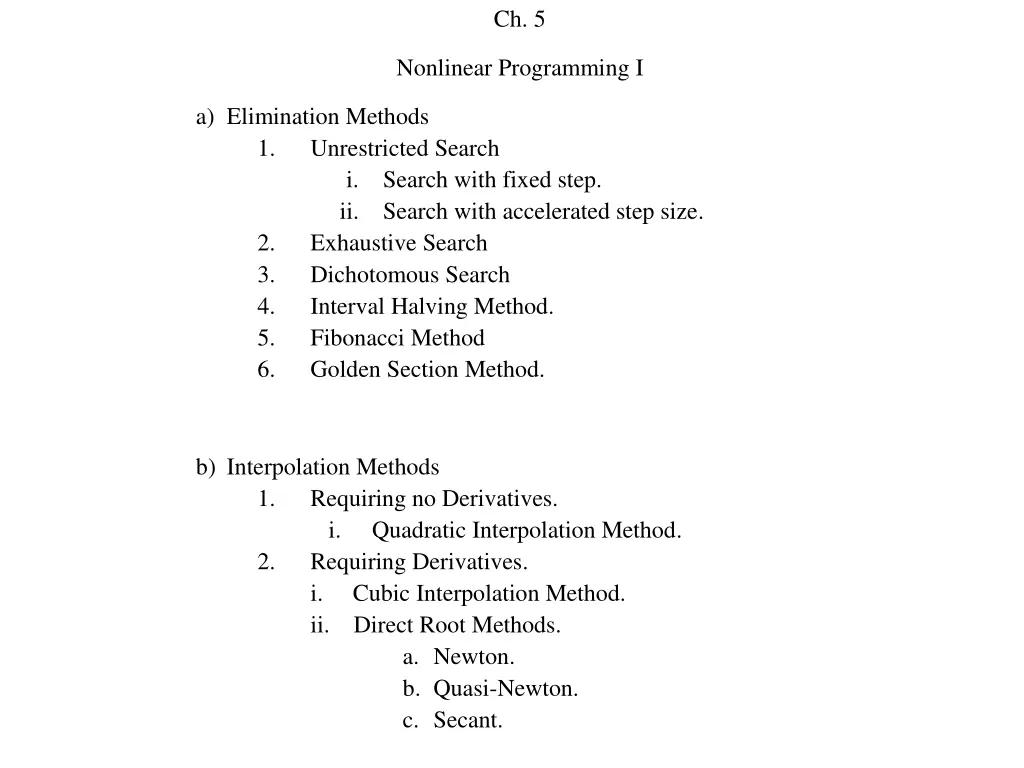
Ch. 5 Nonlinear Programming I a)Elimination Methods 1. Unrestricted Search i.Search with fixed step. ii.Search with accelerated step size. 2. Exhaustive Search 3. Dichotomous Search 4. Interval Halving Method. 5. Fibonacci Method 6. Golden Section Method. b)Interpolation Methods 1. Requiring no Derivatives. i. Quadratic Interpolation Method. 2. Requiring Derivatives. i. Cubic Interpolation Method. ii. Direct Root Methods. a.Newton. b.Quasi-Newton. c.Secant.
7. Direct Root Methods: This group of methods depending on a truth state that; "Since the necessary function ? ? has a minimum ? , three roots-finding methods; the Newton, the quasi-Newton, and the secant methods are discussed below: a. Newton Method: To understand this method, it is preferable to make a review about "Taylor's Series". This series depends on the truth that if one point on a function is known, and the derivatives of this function are also known for that point, then the function can be written as: ? ? = ? = ? ? +? ? ? ? +? ? ? ?2 1! 2! +? ? ? ?3+ .... 3!
Or ?= ??? ? ?? ? ? = ? = ?! ?=0 Now, Newton method states that: For any function ? ? , if a point and second derivatives are known also, then the first three terms of Taylor's series can be written to represent the function ? ? approximately as: ?? on this function and its first ? ?? +1 ? ? = ? ?? + ? ?? 2? ?? 2 (1) ? ?? Then, the first derivative of this function ? ? will be:
Fig. (5-7) as the degree of the Taylor polynomial rises, it approaches the correct function. This image shows sin(x) and its Taylor approximations, polynomials of degree 1, 3, 5, 7, 9, 11 and 13.
?? ? ?? = ? ? = ? ?? + ? ?? ? ?? (2) Since, the substitution of the value of ?? make it equal to zero, because function. The solution of this equation ? will be considered as a new starting point ??+1. Hence, equation (2) can be rearranged as: ? ?? + ? ?? ? ?? + ? ? ?? ??? ?? = 0 ? ? ?? ??? ?? = ? ?? Divide both sides by ? ?? results in: in equation (2) will not ?? is not the minimum of this ? ?? = 0 ? ?? = ? ?? ? ??
Or ? = ?? ? ?? ? ?? Then, this value of ? is considered as ??+1 for the new step as: (??+1) = ?? ? ?? ? ?? Newton or Newton-Raphson Method Ex. 5.12 Find the minimum of the function 0.75 1 + ?2 0.65?tan 11 ? ? = 0.65 .(1) ? Use Newton-Raphson method with the starting point equal to (?1 = 0.1).Assume ? = 0.01.
-1 0.5145 0 -0.1 0.3 -0.287 0.5 -0.34 1 -0.2355 2 -0.103 3 -0.0524 4 -0.03106 ? ? ? 0.6 ? ?( (? ?) ) 0.5 0.4 0.3 0.2 ? ? 0.1 0 -1 -0.5 0 0.5 1 1.5 2 2.5 3 3.5 4 -0.1 -0.2 -0.3 -0.4 The exact shape of the function
1.5? 1 + ?2 2+0.65? 1 + ?2 0.65tan 11 ? ? = (2) ? ? 0.2 -0.49 0.4 0.6 -0.06 0.8 0.187 1 1.5 2 3 4 5 ? ? -0.104 0.1895 0.1308 0.0786 0.03 0.0145 0.0078 0.3 ? ? 0.2 0.1 ? 0 0 1 2 3 4 5 6 -0.1 -0.2 -0.3 -0.4 -0.5 -0.6 The exact shape of the First derivative variation of the objective function
Now, we have only three known quantities about an objective function, these are: i. The exact magnitude of the objective function at a single point (?1= 0.1) is equal to ? ?1 = 0.188197. ii. The first derivative of the objective function at ?1= 0.1 , equal to ( 0.744832). iii.The second derivative of the objective function at ?1= 0.1 equal to 2.68659 . , Solution: The quadratic function extracted from Taylor's series due to the above given information, the objective function will be due to the equation (1):
? ?? +1 ? ? = ? ?? + ? ?? 2? ?? 2 (4) ? ?? ? ? = 0.188197 + ( 0.744832)(? 0.1) +1 2 ? 0.12 2.68659 ? ? = 0.0206157 1.013491? + 1.343295?2 ..(5) ? 0 0.1 0.2 0.3 0.4 0.45 0.5 0.6 0.7 ? ? Sim ? ? Real 0.02 -0.067 -0.128 -0.163 -0.17 -0.163 -0.15 -0.104 -0.031 -0.1 -0.188 -0.25 -0.287 -0.306 -0.309 -0.31 -0.3 -0.29
0.05 0 0 0.1 0.2 0.3 0.4 0.5 0.6 0.7 0.8 -0.05 -0.1 sim -0.15 real -0.2 -0.25 -0.3 -0.35 Taylor's series representation of the real and the simulated objective functions ? ? = 1.013491 + 2.68659? .(6) ? ? = 2.68659 .(7)
Iteration 1 ?1= 0.1,? ?1 = 0.188197,? ?1 = 0.744832,? ?1 = 2.68659 2, 3 ) ( ( 6, 7 ) ?2= ?1 ? ?1 = 0.377241 ? ?1 Convergence check: ? ?2 = 0.13823 > ? Iteration 2 ? ?2 = 0.303279, ? ?2 = 0.13823, ?3= ?2 ? ?2 ? ?2 = 1.57296 = 0.465119 ? ?2
Convergence check: ??4 = 0.0179078 < ? Since the process has converged, the optimum solution is taken as ? 0.480409


 as the degree of the Taylor polynomial rises, it")