Numerical Differentiation and Integration: Basics and Methods
Understand the fundamentals of numerical differentiation and integration in calculus, essential for engineers dealing with changing systems. Learn about forward and central difference formulas, numerical integration techniques like the trapezoidal and Simpson's rules, and non-computer methods for differentiation and integration. Discover how to handle various types of functions, from simple continuous ones to tabulated data, using approximation methods.

Download Presentation

Please find below an Image/Link to download the presentation.
The content on the website is provided AS IS for your information and personal use only. It may not be sold, licensed, or shared on other websites without obtaining consent from the author. If you encounter any issues during the download, it is possible that the publisher has removed the file from their server.
You are allowed to download the files provided on this website for personal or commercial use, subject to the condition that they are used lawfully. All files are the property of their respective owners.
The content on the website is provided AS IS for your information and personal use only. It may not be sold, licensed, or shared on other websites without obtaining consent from the author.
E N D
Presentation Transcript
CHAPTER-V NUMERICAL DIFFERENTIATION & INTEGRATION
CONTENTS: INTRODUCTION FORWARD DIFFERENCE FORMULA CENTRAL DIFFERENCE FORMULA NUMERICAL INTEGRATION TRAPEZOIDAL RULE SIMPSON S RULE
5.1 Introduction: Calculus is mathematics of change. Because engineers must continuously deal with systems and processes that change, calculus is an essential tool of the engineering profession. Standing at the heart of calculus are the related mathematical concepts of differentiation and integration. Mathematically, the derivative represents the rate of change of a dependent variable with respect to an independent variable. If y is the dependent variable and x is the independent variable, the first derivative of y = f(x) w.r.t. to x, represented by dy/dx, is given by
( ) ( ) x + f x x f dy = i i lim dx x 0 x The inverse process to differentiation in calculus is integration. Mathematically, integration is represented by b a ( )dx x = I f which stands for the integral of the function f(x) w.r.t. the independent variable x, evaluated between the limits x = a to x = b. The function f(x) is referred to as the integrand.
Non-Computer Methods for Differentiation and Integration The function to be differentiated or integrated will typically be in one of the following three forms: 1. A simple continuous function such as a polynomial, an exponential, or a trigonometric function. 2. A complicated continuous function that is difficult or impossible to differentiate or integrate directly. 3. A tabulated function where the values of x and f(x) are given at a number of discrete points, as is often the case with experimental or field data.
In the first case, the derivative or integral of a simple function may be evaluated analytically using calculus. For the second case, analytical solutions are often impractical, and sometimes impossible, to obtain. In these instances, as well as in the third case of discrete data, approximate methods must be employed. In the non-computer method for determining derivatives from data, the (x, y) data are tabulated and, for each interval, a simple divided difference y/ x is employed to estimate the slope.
Then these values are plotted as a stepped curve versus x. Next a smooth curve is drawn that attempts to approximate the area under the stepped curve. That is, it is drawn so that visually, the positive and the negative areas are balanced. The rates at given values of x can then be read from the curve. In the same spirit, visually oriented approaches were employed to integrate tabulated data and complicated functions in the pre-computer era. A simple intuitive approach is to plot the function on a grid and count the number of boxes that approximate the area. This number multiplied by the area of each box provides a rough estimate of the total area under the curve.
This estimate can be refined, at the expense of additional effort, by using a finer grid. Another commonsense approach is to divide the area into vertical segments, or strips, with a height equal to the function value at the midpoint of each strip. The area of the rectangles can be then calculated and summed to estimate the total area. In this approach, it is assumed that the value at the midpoint provides a valid approximation of the average height of the function for each strip. As with the grid method, refined estimates are possible by using more (and thinner) strips to approximate the integral.
5.2 Numerical Differentiation : An effective tool for Numerical Differentiation is the Taylor series expansion of f (x) about the point xi. It has the advantage of providing us with information about the error involved in the approximation. Numerical differentiation is not a particularly accurate process. It suffers from a conflict between round off errors (due to limited machine precision) and errors inherent in interpolation. For this reason, a derivative of a function can never be computed with the same precision as the function itself
5.2.1 Lower Order Methods By truncating the second- and higher-derivatives in the Taylor series the following formula for approximating the first derivative, called the first forward difference, is obtained ( ) ( ) x f x f f ( ) x ( ) h ( ) h = + = + +1 i i i f O O h h if Where is referred to as the first forward difference and h is called the step size. The entire term is referred to as a first finite divided difference. f h
Similarly, by truncating the Taylor series between xi-1 and xi, ( ) ( ) ( ) 1 = f x f x f i i ( ) ! 2 f x + 2 i ... x h h i the following formula for approximating the first derivative is obtained ( ) ( ) ( ) h O h f x f x f ( ) x ( ) h = + = + 1 i i i f O i h Where is referred to as the first backward difference. if
A third way to approximate the first derivative is to subtract backward Taylor series expansions (between xi-1 and xi ) from the forward Taylor series expansion (between xi-1 and xi ) resulting in ( ) ( ) ( ) ! 3 ( ) x 3 f = + + + 3 i 2 ... f x f x f x h h + 1 1 i i i from which we obtain ( ) ( ) ( ) h f x f x ( ) x = + 2 1 1 i i f O i 2 h The above equation is a centered difference representation of the first derivative.
Example Consider the function ? ? = ??sin(?) Compute numerical approximations for ? 1 h=0.1,0.01,0.001 using step sizes, ? ? = ? ?sin(?) Using h=0.1 ? 1 =((0.296657)-(0.318477))/(0.2) ? 1 =(-0.0218198)/(0.2) ? 1 =-0.109099 Using h=0.01 ? 1 =((0.308432)-(0.310648))/(0.02) ? 1 =(-0.000221587)/(0.002) ? 1 =-0.110794
Using h=0.001 ? 1 =((0.309449)-(0.30967))/(0.002) ? 1 =(-0.000221587)/(0.02) ? 1 =-0.110794 The true value is: ? 1 =Cos(1) Sin(1) ? ? ? 1 =-0.110794
5.2.2High-Accuracy Differentiation Formulas High-accuracy divided difference formulas can be generated by including additional terms from the Taylor series expansion. For example, the forward Taylor series expansion can be written as ( ) 2 f x ( ) ( ) x ( ) x = + + + 2 i ... f x f f h h + 1 i i i which can be solved for ( ) ( ) x ( ) 2 ( ) h f x f f x ( ) x = + + 2 2 1 i i i f h O i h The result can be truncated by excluding the second- and higher- derivative terms and were thus left with a final result
( ) ( ) x f x f ( ) x ( ) h = + +1 i i f O i h We can retain the second-derivative term by substituting the following approximation of the second derivative ( ) ( 2 ) ( ) x + 2 f x f x f ( ) x ( ) h = + + + 2 1 i i i f O i h into Eq. 2 to yield ( ) ( ) x ( ) ( ) ( ) x + ( ) h 2 f x f f x f x f ( ) x = + + + + 2 1 2 1 i i i i i f h O i 2 h 2 h
collecting terms ( ) ( h ) ( ) x + ( ) h 4 3 f x f x f ( ) x = + + + 2 2 1 i i i f O i 2 Notice that the inclusion of the second-derivative term has improved the accuracy to O (h2). Similar improved versions can be developed for the backward and centered formulas as well as for the approximations of the higher derivatives. The formulas are given below.
Forward Finite-divided Difference Formulas First Derivative ( ) x f i = Error ( ) h O f ( ) ( ) x f x +1 i i h ) ( ) h ( ( h ) ( ) x + 4 3 f x f 2 x f 2 O ( ) x = + + 2 1 i i i f i Second Derivative ( ) h ( ) ( 2 ) ( ) x + 2 f x f x f 2 O ( ) x = + + 2 1 i i i f i h ( ( ) ) ( ) ( ) x + + 4 5 2 f x f x f x f ( ) x ( ) h = + + + 3 2 1 i i i i f 2 O i 2 h
Third Derivative ( ) x f i = ( ) ( ) h ( ) ( ) x + 3 3 f x f x f x f + + + 3 2 1 i i i i 3 ( ) ( ) ( ) ( ) ( ) x + + 3 14 24 18 5 f x f x f x f x f ( ) x = + + + + 4 3 2 1 i i i i i f i 3 2 h Fourth Derivative f x f i = ( ) ( ) ( 4 ) ( ) ( ) x + + 4 6 4 x f x f x f x f ( )( ) + + + + 4 4 3 2 1 i i i i i h ) ( ) ( ( ) 4 ( ) ( ) ( ) x + + + 2 11 24 26 14 3 f x f x f x f x f x f ( )( ) = + + + + + 4 5 4 3 h 2 1 i i i i i i f x i
Look on the handout for Backward Finite-divided Difference Formulas Centered Finite-divided Difference Formulas
5.3Newton-Cotes integration formulas The Newton-Cotes formulas are the most common numerical integration schemes. They are based on the strategy of replacing a complicated function or tabulated data with an approximating function that is easy to integrate: ( ) dx x f I a b b ( )dx x = f n a where fn(x) = a polynomial of the form ( ) n x f = + + + + 1 n n ... a a x a x a x 0 1 1 n n where n is the order of the polynomial.
The integral can be approximated by one polynomial or using a series of polynomials applied piecewise to the function or date over segments of constant length. Closed and open forms of the Newton-Cotes formulas are available. The closed forms are those where the data points at the beginning and end of the limits of integration are known. The open forms have integration limits that extend beyond the range of the data.
1.The Trapezoidal Rule The trapezoidal rule is the first of the Newton-Cotes closed integration formulas. It corresponds to the case where the polynomial in Eq. is first-order: b b ( ) x ( )dx x = I f dx f 1 a a The straight line passing through the two points (a, f(a)) and (b, f(b)) is given by ( ) ( ) a f x f + = 1 ( ) b ( )( f b f a ) a x a
The area under this straight line is an estimate of the integral of f(x) between the limits a and b: ( ) b ( )( b a f b f a ( ) a ) dx = + I f x a a The result of the integration is ( ) a ( ) b + f f ( ) = I b a 2 which is called the trapezoidal rule.
Error of the Trapezoidal Rule When we employ the integral under a straight line to approximate the integral under the curve, we obviously can incur an error that may be substantial. An estimate of the local truncation error of a single application of the trapezoidal rule is 1 ( )( )3 = Et f b a 12 where lies somewhere in the interval from a to b.
Multiple-Application of Trapezoidal Rule One way to improve the accuracy of the trapezoidal rule is to divide the integration interval from a to b into a number of segments and apply the method to each segment. The areas of the individual segments can then be added to yield the integral for the entire interval. The resulting equations are called multiple-application, or composite, integration formulas. Considering n + 1 equally spaced base points (x0, x1, x2, ..., xn), and n segments of equal width:
b a = h n If a and b are designated as x0 and xn, respectively, the total integral can be represented as x x x n 1 2 ( ) x ( ) x ( )dx x n = + + + ... I f dx f dx f x x x 0 1 1 Substituting the trapezoidal rule for each interval yields ( ) x ( ) x ( ) ( ) x ( ) x ( ) x + + + f f f x f f f = + + + 0 1 1 n n 1 2 ... I h h h 2 2 2
or, grouping terms, 1 n h ( ) ( ) x ( ) = i = + + 2 I f x f f x 0 i n 2 1 or, It can be expressed in the following form, 1 n = ( ) ( ) x ( ) + + 2 f x f f x 0 i n ( ) = 1 i I b a 2 n
An error for the multiple-application trapezoidal rule can be obtained by summing the individual errors for each segment to give ( ) ( ) = i n 1 12 n b a 3 = E f t i where f"( i) is the second derivative at a point i located in segment i. This result can be simplified by estimating the mean or the average value of the second derivative for the entire interval as
n ( ) = f i 1 i f n ( ) and Eq. 5.25 can be rewritten as Therefore f f n i ( ) 3 b 12 a = Ea f 2 n Thus, if the number of segment is doubled, the truncation error will be quartered.
Example Numerically approximate the integral by using the trapezoidal rule with m = 1, 2, 4, 8, and 16 subintervals. For m = 1
For m = 2 For m = 4 follow the same procedure for m = 8 and 16
5.3.2 Simpson's Rules Aside from applying the trapezoidal rule with finer segmentation, another way to obtain a more accurate estimate of an integral is to use higher-order polynomial to connect the points. For example, if there is an extra point midway between f(a) and f(b), the three points can be connected with a parabola. If there are two points equally spaced between f(a) and f(b), the four points can be connected with a third-order polynomial.
The formulas that result from taking the integrals under these polynomials are called Simpson's rules. i) Simpson's 1/3 Rule Simpson's 1/3 rule results when a second-order interpolating polynomial is substituted into Eq. 5.13: ( ) dx x f I a b b ( )dx x = f 2 a If a and b are designated as x0 and x2 and f2(x) is represented by a second-order Lagrange polynomial, the integral becomes
( x )( )( ) ( x )( )( ) ( x )( )( ) x x x x x x x x x x x x x x 2 ( ) x ( ) x ( ) dx x 2 = + + 0 2 1 2 1 2 I f f f ( ) ( ) ( ) 0 1 x x x x x x x x x 0 1 0 2 0 1 0 2 0 1 0 2 After integration and algebraic manipulation, the following formula results h ( ) x ( ) x ( ) x + + 4 I f f f 0 1 2 3 where, for this case, . This equation is known as Simpson's 1/3 rule.
Simpson's 1/3 rule can also be expressed in the following format ( ) x ( ) 6 ( ) x + + 4 f f x f ( ) 0 1 2 I b a Where a=x0, b=x2 and x1= the point midway between a and b, which is given by (b+a)/2. Notice that, according to the above equation, the middle point is weighted two-thirds and the two end points by one- sixth.
It can be shown that a single-segment application of Simpson's 1/3 rule has a truncation error of 1 ( )( ) = 5 4 Et h f 90 ( ) 2 = because h b a ( ) 5 b a ( )( ) = 4 Et f 2880 where lies somewhere in the interval from a to b. Thus, Simpson's 1/3 rule is more accurate that the trapezoidal rule.
Multiple Application of Simpson's 1/3 Rule Just as with the trapezoidal rule, Simpson's rule can be improved by dividing the integration interval into a number of segments of equal width: b a = h n The total integration can be represented as x x x n 2 4 ( ) x ( ) x ( )dx x n = + + + ... I f dx f dx f 2 x x x 0 2
Substituting Simpson's 1/3 rule for the individual integral yields ( ) x ( ) 6 x ( ) x ( ) x ( ) 6 ( ) x + + + + 4 4 f f x f f f x f + + 0 1 2 2 3 4 2 2 ... I h h ( ) ( 6 ) ( ) x + + 4 f f x f + 2 1 n n n 2 h combining terms, ( ) x 1 2 n = n = ( ) x ( ) x ( ) + + + 4 2 f f f f x 0 i j n ( ) 5 , 3 , 1 6 , 4 , 2 i j I b a 3 n
An error estimate for the multiple-application Simpson's rule is obtained in the same fashion as for the trapezoidal rule by summing the individual errors for the segments and averaging the derivative to yield ( ) 4 5 b a ( ) 4 = Ea f 180 n ( ) 4 Where is the average fourth derivative for the interval. f
Example Numerically approximate the integral by using Simpson's rule with m = 1, 2, 4, and 8. For m = 1
For m = 2 For m = 4
Simpson's 3/8 Rule In a similar manner to the derivation of the trapezoidal and Simpson's 1/3 rule, a third-order Lagrange polynomial can be fit to four points and integrated: b b ( ) x ( )dx x = I f dx f 3 ( ) 3 = h b a a a to yield ( ) ( ) x ( ) ( ) + + + 3 3 f x f f x f x 3 h 0 1 2 3 I 8 8
( ) 3 = h b a Where This equation is called Simpson's 3/8 rule because h is multiplied by 3/8. It is the third Newton-Cotes closed integration formula. The 3/8 rule can also be expressed in the following form: ( ) x ( ) x ( ) x ( ) x + + + 3 3 f f f f ( ) 0 1 2 3 I b a 8
Thus, the two interior points are given weight's are given weights of three-eighths, whereas the end points are weighted with one-eighth. Simpson's 3/8 rule has an error of ( ) 5 b a ( )( ) = 4 Et f 6480
Simpson's 1/3 rule is usually the method of preference because it attains third-order accuracy with three points rather than the four points required for the 3/8 version. However, the 3/8 rule has utility when the number of segments is odd.
Example Numerically approximate the integral by using Simpson's 3/8 rule with m = 1, 2, 4. For m = 1 For m = 2


")